Reproducibility with original data

This tutorial demonstrates deconvolution to map cell types of the mouse cortex from sc-RNA-seq data to Visium data using Pysodb and Tangram.

A reference paper can be found at https://www.nature.com/articles/s41592-021-01264-7.

This tutorial refers to the following tutorial at https://squidpy.readthedocs.io/en/stable/external_tutorials/tutorial_tangram.html. At the same time, the way of loadding data is modified by using Pysodb.

The single cell data utilized in the tutorial can be accessed directly from Figshare at https://figshare.com/articles/dataset/Visium/22332667.

Import packages and set configurations

# Import several Python packages, including:
# scanpy: a Python package for single-cell RNA sequencing analysis
import scanpy as sc
# squidpy: a Python package for spatial transcriptomics analysis
import squidpy as sq
# numpy: a Python package for scientific computing with arrays
import numpy as np
# pandas: a Python package for data manipulation and analysis
import pandas as pd

When encountering the Error “No module named ‘squidpy’”, users should activate the virtual environment at the terminal and execute “pip install squidpy”.

# Import tangram for spatial deconvolution
import tangram as tg

# print a header message, and the version of the squidpy and tangram packages
sc.logging.print_header()
print(f"squidpy=={sq.__version__}")
print(f"tangram=={tg.__version__}")

scanpy==1.9.3 anndata==0.8.0 umap==0.5.3 numpy==1.22.4 scipy==1.9.1 pandas==1.5.3 scikit-learn==1.2.2 statsmodels==0.13.5 python-igraph==0.10.4 pynndescent==0.5.8
squidpy==1.2.3
tangram==1.0.4

import matplotlib.pyplot as plt
from matplotlib.colors import ListedColormap
import palettable

adjusted_qualitative_colors = [
    '#5e81ac', '#f47b56', '#7eaca9', '#e28b90', '#ab81bd', '#b68e7e', '#df8cc4', '#7f7f7f', '#bcbd22', '#17becf',
    '#aec7e8', '#ffbb78', '#98df8a', '#ff9896', '#c5b0d5', '#c49c94', '#f7b6d2', '#c7c7c7', '#dbdb8d', '#9edae5',
    '#393b79', '#5254a3', '#6b6ecf', '#9c9ede', '#637939', '#8ca252', '#b5cf6b', '#cedb9c', '#8c6d31', '#bd9e39'
]

# Create adjusted custom qualitative colormap
adjusted_qualitative_cmap = ListedColormap(adjusted_qualitative_colors)

# Example of using the custom colormap with Scanpy
# sc.pl.umap(adata, color='gene_name', cmap=adjusted_qualitative_cmap)
cmp_ct = palettable.cartocolors.qualitative.Safe_10.mpl_colors

When encountering the Error “No module named ‘palettable’”, users should activate the virtual environment at the terminal and execute “pip install pip install palettable”.

Load a single cell dataset

# Load the reference single cell dataset
# The input sc data has been normalized and log-transformed
adata_sc = sc.read_h5ad('data/Visium/sc_mouse_cortex.h5ad')

# Print out the metadata of adata_sc
adata_sc

AnnData object with n_obs × n_vars = 21697 × 36826
    obs: 'sample_name', 'organism', 'donor_sex', 'cell_class', 'cell_subclass', 'cell_cluster', 'n_genes_by_counts', 'log1p_n_genes_by_counts', 'total_counts', 'log1p_total_counts', 'pct_counts_in_top_50_genes', 'pct_counts_in_top_100_genes', 'pct_counts_in_top_200_genes', 'pct_counts_in_top_500_genes', 'total_counts_mt', 'log1p_total_counts_mt', 'pct_counts_mt', 'n_counts'
    var: 'mt', 'n_cells_by_counts', 'mean_counts', 'log1p_mean_counts', 'pct_dropout_by_counts', 'total_counts', 'log1p_total_counts', 'n_cells', 'highly_variable', 'highly_variable_rank', 'means', 'variances', 'variances_norm'
    uns: 'cell_class_colors', 'cell_subclass_colors', 'hvg', 'neighbors', 'pca', 'umap'
    obsm: 'X_pca', 'X_umap'
    varm: 'PCs'
    obsp: 'connectivities', 'distances'

# Visualize a UMAP projection colored by cell_subclass
fig,ax = plt.subplots(figsize=(4,4))
sc.pl.embedding(adata_sc,basis='umap',color=['cell_subclass'],ax=ax,show=False,palette=adjusted_qualitative_colors,s=5)

<Axes: title={'center': 'cell_subclass'}, xlabel='UMAP1', ylabel='UMAP2'>

Streamline development of loading spatial data with Pysodb

# Import pysodb package
# Pysodb is a Python package that provides a set of tools for working with SODB databases.
# SODB is a format used to store data in memory-mapped files for efficient access and querying.
# This package allows users to interact with SODB files using Python.
import pysodb

# Initialization
sodb = pysodb.SODB()

# Define the name of the dataset_name and experiment_name
dataset_name = 'Biancalani2021Deep'
experiment_name = 'visium_fluo_crop'
# Load a specific experiment
# It takes two arguments: the name of the dataset and the name of the experiment to load.
# Two arguments are available at https://gene.ai.tencent.com/SpatialOmics/.
adata_st = sodb.load_experiment(dataset_name,experiment_name)

load experiment[visium_fluo_crop] in dataset[Biancalani2021Deep]

adata_st

AnnData object with n_obs × n_vars = 704 × 16562
    obs: 'in_tissue', 'array_row', 'array_col', 'n_genes_by_counts', 'log1p_n_genes_by_counts', 'total_counts', 'log1p_total_counts', 'pct_counts_in_top_50_genes', 'pct_counts_in_top_100_genes', 'pct_counts_in_top_200_genes', 'pct_counts_in_top_500_genes', 'total_counts_MT', 'log1p_total_counts_MT', 'pct_counts_MT', 'n_counts', 'leiden', 'cluster'
    var: 'gene_ids', 'feature_types', 'genome', 'MT', 'n_cells_by_counts', 'mean_counts', 'log1p_mean_counts', 'pct_dropout_by_counts', 'total_counts', 'log1p_total_counts', 'n_cells', 'highly_variable', 'highly_variable_rank', 'means', 'variances', 'variances_norm', 'dispersions', 'dispersions_norm'
    uns: 'cluster_colors', 'hvg', 'leiden', 'leiden_colors', 'log1p', 'moranI', 'neighbors', 'pca', 'spatial', 'spatial_neighbors', 'umap'
    obsm: 'X_pca', 'X_umap', 'spatial'
    varm: 'PCs'
    obsp: 'connectivities', 'distances', 'spatial_connectivities', 'spatial_distances'

# Create a spatial scatter plot colored by cluster label
cmp_ct = palettable.cartocolors.qualitative.Pastel_10.mpl_colors
cmp_ct.append('gray')
cmp_ct_cmp = ListedColormap(cmp_ct)

ax = sq.pl.spatial_scatter(adata_st,color='cluster',size=1.2,palette=cmp_ct_cmp)

Preparation

# Visualize embedding base on 'spatial' with points colored by 'cluster' label
sc.pl.embedding(adata_st,basis='spatial',color='cluster')

# select a subset based on the "Cortex_{i}" of 'adata_st.obs.cluster'
# And creates a copy of the resulting subset

adata_st = adata_st[
    adata_st.obs.cluster.isin([f"Cortex_{i}" for i in np.arange(1, 5)])
].copy()

# Visualize embedding base on 'spatial' with points colored by a new 'cluster' label
sc.pl.embedding(adata_st,basis='spatial',color='cluster')

cmp_ct = palettable.cartocolors.qualitative.Pastel_10.mpl_colors
cmp_ct_cmp = ListedColormap(cmp_ct)

ax = sq.pl.spatial_scatter(adata_st,color='cluster',size=1.2,palette=cmp_ct_cmp)

# Perform differential gene expression analysis across 'cell_subclasses' in 'adata_sc'
sc.tl.rank_genes_groups(adata_sc, groupby="cell_subclass", use_raw=False)

WARNING: Default of the method has been changed to 't-test' from 't-test_overestim_var'

# Create a Pandas DataFrame called "markers_df" by extracting the top 100 differentially expressed genes from 'adata_sc'
markers_df = pd.DataFrame(adata_sc.uns["rank_genes_groups"]["names"]).iloc[0:100, :]
# Create a NumPy array called "genes_sc" by extracting the unique values from the "value" column of a melted version of the "markers_df"
genes_sc = np.unique(markers_df.melt().value.values)
# Extracte the names of genes from "adata_st"
genes_st = adata_st.var_names.values
# Create a Python list called "genes"
# Contain the intersection of genes identified as differentially expressed in  "genes_sc" and genes detected in "genes_st".
genes = list(set(genes_sc).intersection(set(genes_st)))
# The length of "genes"
len(genes)

1281

Perform Tangram for alignment

# Use the Tangram to align the gene expression profiles of "adata_sc" and "adata_st" based on the shared set of genes identified by the intersection of "genes_sc" and "genes_st".
tg.pp_adatas(adata_sc, adata_st, genes=genes)

INFO:root:1280 training genes are saved in `uns``training_genes` of both single cell and spatial Anndatas.
INFO:root:14785 overlapped genes are saved in `uns``overlap_genes` of both single cell and spatial Anndatas.
INFO:root:uniform based density prior is calculated and saved in `obs``uniform_density` of the spatial Anndata.
INFO:root:rna count based density prior is calculated and saved in `obs``rna_count_based_density` of the spatial Anndata.

# Use the map_cells_to_space function from the tangram to map cells from "adata_sc" onto "adata_st".
# The mapping use "cells" mode, which assign each cell from adata_sc to a location within the spatial transcriptomics space based on its gene expression profile.
ad_map = tg.map_cells_to_space(
    adata_sc,
    adata_st,
    mode="cells",
    # target_count=adata_st.obs.cell_count.sum(),
    # density_prior=np.array(adata_st.obs.cell_count) / adata_st.obs.cell_count.sum(),
    num_epochs=1000,
    device="cpu",
)

INFO:root:Allocate tensors for mapping.
INFO:root:Begin training with 1280 genes and rna_count_based density_prior in cells mode...
INFO:root:Printing scores every 100 epochs.

Score: 0.613, KL reg: 0.001
Score: 0.733, KL reg: 0.000
Score: 0.736, KL reg: 0.000
Score: 0.737, KL reg: 0.000
Score: 0.737, KL reg: 0.000
Score: 0.737, KL reg: 0.000
Score: 0.737, KL reg: 0.000
Score: 0.737, KL reg: 0.000
Score: 0.738, KL reg: 0.000
Score: 0.738, KL reg: 0.000

INFO:root:Saving results..

ad_map

AnnData object with n_obs × n_vars = 21697 × 324
    obs: 'sample_name', 'organism', 'donor_sex', 'cell_class', 'cell_subclass', 'cell_cluster', 'n_genes_by_counts', 'log1p_n_genes_by_counts', 'total_counts', 'log1p_total_counts', 'pct_counts_in_top_50_genes', 'pct_counts_in_top_100_genes', 'pct_counts_in_top_200_genes', 'pct_counts_in_top_500_genes', 'total_counts_mt', 'log1p_total_counts_mt', 'pct_counts_mt', 'n_counts'
    var: 'in_tissue', 'array_row', 'array_col', 'n_genes_by_counts', 'log1p_n_genes_by_counts', 'total_counts', 'log1p_total_counts', 'pct_counts_in_top_50_genes', 'pct_counts_in_top_100_genes', 'pct_counts_in_top_200_genes', 'pct_counts_in_top_500_genes', 'total_counts_MT', 'log1p_total_counts_MT', 'pct_counts_MT', 'n_counts', 'leiden', 'cluster', 'uniform_density', 'rna_count_based_density'
    uns: 'train_genes_df', 'training_history'

# Project "Cell_subclass" annotations from a single-cell RNA sequencing (scRNA-seq) dataset onto a spatial transcriptomics dataset, based on a previously computed cell-to-space mapping
tg.project_cell_annotations(ad_map, adata_st, annotation="cell_subclass")

INFO:root:spatial prediction dataframe is saved in `obsm` `tangram_ct_pred` of the spatial AnnData.

# Transfer cell type predictions from the AnnData object's ‘obsm’ attribute (adata_st.obsm['tangram_ct_pred']) to its observation metadata (adata_st.obs)
for ct in adata_st.obsm['tangram_ct_pred'].columns:
    adata_st.obs[ct] = np.array(adata_st.obsm['tangram_ct_pred'][ct].values)

# Print adata_st.obsm['tangram_ct_pred']
adata_st.obsm['tangram_ct_pred']

	Pvalb	L4	Vip	L2/3 IT	Lamp5	NP	Sst	L5 IT	Oligo	L6 CT	...	L5 PT	Astro	L6b	Endo	Peri	Meis2	Macrophage	CR	VLMC	SMC
AAATGGCATGTCTTGT-1	7.004985	1.548934	6.902157	0.001669	4.129408	4.114066	3.220240	3.820235	0.288011	8.503994	...	7.850845	2.551129	0.000456	0.421885	0.000057	0.000061	1.297545	0.071324	0.129917	0.685547
AACAACTGGTAGTTGC-1	4.209501	0.000783	13.903717	0.192844	4.696000	3.499797	6.033508	9.985192	0.456206	2.967823	...	7.369421	1.928740	0.928254	0.526186	0.107533	0.000130	0.547133	0.079866	0.000185	0.275435
AACAGGAAATCGAATA-1	4.682822	0.526977	7.370772	0.571306	6.074437	1.000437	7.754989	5.081327	0.396358	15.313167	...	1.394540	2.027951	0.473381	0.544031	0.228793	1.153768	0.685693	0.000441	0.000177	0.262540
AACCCAGAGACGGAGA-1	8.718892	4.313211	4.679913	3.914560	8.065018	0.000336	7.402516	9.868730	0.476459	2.293070	...	0.230093	2.908436	0.000443	0.586561	0.000053	0.475399	0.902312	0.000050	0.578500	0.581497
AACCGTTGTGTTTGCT-1	8.815555	5.802182	4.890625	1.156238	5.074965	0.487821	8.204679	14.393296	1.581857	0.000475	...	2.226670	1.070311	1.225542	1.491899	0.074052	0.000590	0.215931	0.055336	0.000093	0.551992
...	...	...	...	...	...	...	...	...	...	...	...	...	...	...	...	...	...	...	...	...	...
TTGGATTGGGTACCAC-1	5.916564	2.063360	13.772404	1.952126	2.691196	2.123059	12.909450	9.272922	0.410706	0.005365	...	6.397924	2.403446	0.000223	0.458006	0.038058	0.000083	0.227499	0.018278	0.252095	0.642331
TTGGCTCGCATGAGAC-1	2.514913	4.281378	4.322568	10.849935	8.974291	0.000461	13.464813	9.720862	0.139286	0.609628	...	0.000646	0.838765	0.076363	0.416698	0.059241	0.025889	0.272974	0.000290	0.260999	0.389371
TTGTATCACACAGAAT-1	3.621018	0.001693	6.560889	1.507911	5.990241	4.790297	8.296551	8.652060	0.563544	5.002628	...	3.863253	0.750675	1.071313	0.396808	0.058517	0.034917	0.193589	0.000341	0.272419	0.238980
TTGTGGCCCTGACAGT-1	9.345364	2.639463	9.780218	0.001793	0.349541	0.998307	4.595858	5.134462	0.792228	7.001610	...	4.198365	2.206220	1.493556	0.653867	0.068874	0.000080	0.696597	0.000134	0.323000	0.212188
TTGTTAGCAAATTCGA-1	4.926483	22.468429	5.517707	0.864528	1.313571	0.000482	5.217501	12.868741	0.667749	0.740462	...	0.435651	1.406598	0.000301	0.509059	0.103536	0.436183	0.113370	0.000399	0.191394	0.058175

324 rows × 23 columns

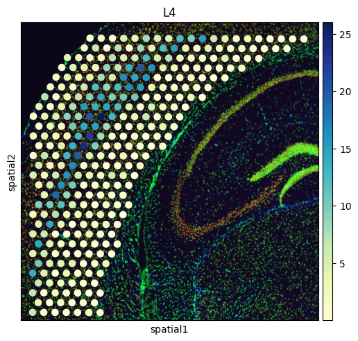
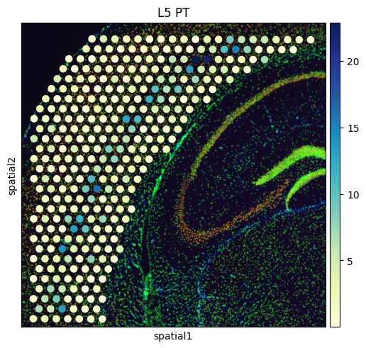
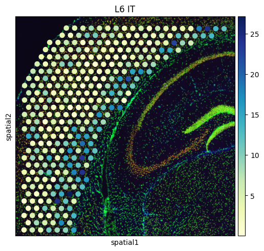
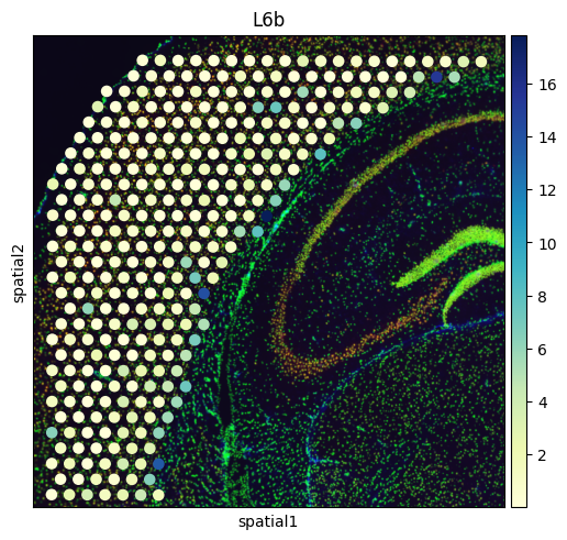
# Create a spatial embedding plot that visualizes the distribution of diverse cell types
from palettable.colorbrewer.sequential import YlGnBu_9
to_plot_list = ['VLMC','Astro',"L2/3 IT", "L4", "L5 IT", "L5 PT", "L6 CT", "L6 IT", "L6b"]

for to_plot in to_plot_list:
    sq.pl.spatial_scatter(
        adata_st,

        color=to_plot,
        cmap=YlGnBu_9.mpl_colormap
    )
    to_plot = to_plot.replace('/','_')
    to_plot = to_plot.replace(' ','_')