Application with new data
This tutorial demonstrates deconvolution on new ST human pancreatic cancer data using Pysodb and Tangram.
This tutorial refers to the following tutorial at https://squidpy.readthedocs.io/en/stable/external_tutorials/tutorial_tangram.html. At the same time, the way of loadding data is modified by using Pysodb.
The single cell data utilized in the tutorial is directly available at https://figshare.com/articles/dataset/PDAC/22332574.
Import packages and set configurations
[1]:
# Import several Python packages, including:
# scanpy: a Python package for single-cell RNA sequencing analysis
import scanpy as sc
# squidpy: a Python package for spatial transcriptomics analysis
import squidpy as sq
# numpy: a Python package for scientific computing with arrays
import numpy as np
# pandas: a Python package for data manipulation and analysis
import pandas as pd
# anndata: a Python package for handling annotated data objects in genomics
import anndata as ad
When encountering the Error “No module named ‘squidpy’”, users should activate the virtual environment at the terminal and execute “pip install squidpy”.
[2]:
# Import tangram for spatial deconvolution
import tangram as tg
[3]:
# Print a header message, and the version of the squidpy and tangram packages
sc.logging.print_header()
print(f"squidpy=={sq.__version__}")
print(f"tangram=={tg.__version__}")
scanpy==1.9.3 anndata==0.8.0 umap==0.5.3 numpy==1.22.4 scipy==1.9.1 pandas==1.5.3 scikit-learn==1.2.2 statsmodels==0.13.5 python-igraph==0.10.4 pynndescent==0.5.8
squidpy==1.2.3
tangram==1.0.4
[4]:
import matplotlib.pyplot as plt
from matplotlib.colors import ListedColormap
import palettable
# Define a list of color hex codes
adjusted_qualitative_colors = [
    '#5e81ac', '#f47b56', '#7eaca9', '#e28b90', '#ab81bd', '#b68e7e', '#df8cc4', '#7f7f7f', '#bcbd22', '#17becf',
    '#aec7e8', '#ffbb78', '#98df8a', '#ff9896', '#c5b0d5', '#c49c94', '#f7b6d2', '#c7c7c7', '#dbdb8d', '#9edae5',
    '#393b79', '#5254a3', '#6b6ecf', '#9c9ede', '#637939', '#8ca252', '#b5cf6b', '#cedb9c', '#8c6d31', '#bd9e39'
]

# Create adjusted custom qualitative colormap
adjusted_qualitative_cmap = ListedColormap(adjusted_qualitative_colors)

# Example of using the custom colormap with Scanpy
# sc.pl.umap(adata, color='gene_name', cmap=adjusted_qualitative_cmap)

# Create a list of 10 soft pastel colormap
cmp_ct = palettable.cartocolors.qualitative.Pastel_10.mpl_colors
When encountering the Error “No module named ‘palettable’”, users should activate the virtual environment at the terminal and execute “pip install pip install palettable”.
Load a single cell dataset
[5]:
# Read CSV files
#pd_sc = pd.read_csv('data/pdac/sc_data.csv')
#pd_sc_meta = pd.read_csv('data/pdac/sc_meta.csv')
pd_sc = pd.read_csv('data/pdac/sc_data.csv')
pd_sc_meta = pd.read_csv('data/pdac/sc_meta.csv')
[6]:
# Set the index
pd_sc = pd_sc.set_index('Unnamed: 0')
pd_sc_meta = pd_sc_meta.set_index('Cell')
[7]:
# Extract gene names and cell identifiers
sc_genes = np.array(pd_sc.index)
sc_obs = np.array(pd_sc.columns)
# Transpose the expression data
sc_X = np.array(pd_sc.values).transpose()
[8]:
#Create an AnnData object
adata_sc = ad.AnnData(sc_X)
adata_sc.var_names = sc_genes
adata_sc.obs_names = sc_obs
# Add cell type information to the AnnData object
adata_sc.obs['CellType'] = pd_sc_meta['Cell_type'].values
[9]:
# Print out the metadata of adata_sc
adata_sc
[9]:
AnnData object with n_obs × n_vars = 1926 × 19104
    obs: 'CellType'
[10]:
# Preprocess scRNA-seq data by selecting highly variable genes, normalizing expression values per cell, and applying a log transformation
sc.pp.highly_variable_genes(adata_sc, flavor="seurat_v3", n_top_genes=3000)
sc.pp.normalize_total(adata_sc, target_sum=1e4)
sc.pp.log1p(adata_sc)
[11]:
# Perform dimensionality reduction and constructs a neighborhood graph
sc.pp.pca(adata_sc)
sc.pp.neighbors(adata_sc)
sc.tl.umap(adata_sc)
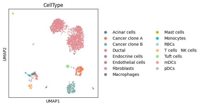
[12]:
# Visualize the UMAP results
fig,ax = plt.subplots(figsize=(4,4))
sc.pl.embedding(adata_sc,basis='umap',color=['CellType'],ax=ax,show=False,palette=adjusted_qualitative_colors,s=20)
[12]:
<Axes: title={'center': 'CellType'}, xlabel='UMAP1', ylabel='UMAP2'>
Streamline development of loading spatial data with Pysodb
[13]:
# Import pysodb package
# Pysodb is a Python package that provides a set of tools for working with SODB databases.
# SODB is a format used to store data in memory-mapped files for efficient access and querying.
# This package allows users to interact with SODB files using Python.
import pysodb
[14]:
# Initialization
sodb = pysodb.SODB()
[15]:
# Define the name of the dataset_name and experiment_name
dataset_name = 'moncada2020integrating'
experiment_name = 'GSM3036911_spatial_transcriptomics'
# Load a specific experiment
# It takes two arguments: the name of the dataset and the name of the experiment to load.
# Two arguments are available at https://gene.ai.tencent.com/SpatialOmics/.
adata_st = sodb.load_experiment(dataset_name,experiment_name)
load experiment[GSM3036911_spatial_transcriptomics] in dataset[moncada2020integrating]
[16]:
# Preprocess data
sc.pp.highly_variable_genes(adata_st, flavor="seurat_v3", n_top_genes=3000)
sc.pp.normalize_total(adata_st, target_sum=1e4)
sc.pp.log1p(adata_st)
[17]:
# Dimensionality reduction and neighborhood graph construction
sc.pp.pca(adata_st)
sc.pp.neighbors(adata_st)
sc.tl.umap(adata_st)
# Cluster cells using the Leiden algorithm
sc.tl.leiden(adata_st,resolution=0.7)
[18]:
# Visualize the spatial embedding
ax = sc.pl.embedding(adata_st,basis='spatial',color=['leiden'],palette=cmp_ct,show=False)
ax.axis('equal')
[18]:
(0.5999999999999999, 31.4, 6.7, 35.3)

Preparation
[19]:
# Perform differential gene expression analysis across 'CellType' in 'adata_sc'
sc.tl.rank_genes_groups(adata_sc, groupby="CellType", use_raw=False)
WARNING: Default of the method has been changed to 't-test' from 't-test_overestim_var'
[20]:
# Extract the top 100 marker genes per cell type from single-cell dataset
markers_df = pd.DataFrame(adata_sc.uns["rank_genes_groups"]["names"]).iloc[0:100, :]
# Find unique marker genes
genes_sc = np.unique(markers_df.melt().value.values)
# Get gene names from spatial transcriptomics dataset
genes_st = adata_st.var_names.values
# Find the intersection of gene sets
genes = list(set(genes_sc).intersection(set(genes_st)))
# The length of "genes"
len(genes)
[20]:
1103
Perform Tangram for alignment
[21]:
# Use the Tangram to align the gene expression profiles of "adata_sc" and "adata_st" based on the shared set of genes identified by the intersection of "genes_sc" and "genes_st".
tg.pp_adatas(adata_sc, adata_st, genes=genes)
INFO:root:1079 training genes are saved in `uns``training_genes` of both single cell and spatial Anndatas.
INFO:root:13775 overlapped genes are saved in `uns``overlap_genes` of both single cell and spatial Anndatas.
INFO:root:uniform based density prior is calculated and saved in `obs``uniform_density` of the spatial Anndata.
INFO:root:rna count based density prior is calculated and saved in `obs``rna_count_based_density` of the spatial Anndata.
[22]:
# Use the map_cells_to_space function from the tangram to map cells from "adata_sc")" onto "adata_st".
# The mapping use "cells" mode, which assign each cell from adata_sc to a location within the spatial transcriptomics space based on its gene expression profile.
ad_map = tg.map_cells_to_space(
    adata_sc,
    adata_st,
    mode="cells",
    # target_count=adata_st.obs.cell_count.sum(),
    # density_prior=np.array(adata_st.obs.cell_count) / adata_st.obs.cell_count.sum(),
    num_epochs=1000,
    device="cpu",
)
INFO:root:Allocate tensors for mapping.
INFO:root:Begin training with 1079 genes and rna_count_based density_prior in cells mode...
INFO:root:Printing scores every 100 epochs.
Score: 0.340, KL reg: 0.113
Score: 0.587, KL reg: 0.001
Score: 0.591, KL reg: 0.001
Score: 0.592, KL reg: 0.001
Score: 0.592, KL reg: 0.001
Score: 0.592, KL reg: 0.001
Score: 0.592, KL reg: 0.001
Score: 0.592, KL reg: 0.001
Score: 0.592, KL reg: 0.001
Score: 0.592, KL reg: 0.001
INFO:root:Saving results..
[23]:
# Project "CellType" annotations from a single-cell RNA sequencing (scRNA-seq) dataset onto a spatial transcriptomics dataset, based on a previously computed cell-to-space mapping
tg.project_cell_annotations(ad_map, adata_st, annotation="CellType")
INFO:root:spatial prediction dataframe is saved in `obsm` `tangram_ct_pred` of the spatial AnnData.
[24]:
# Create new columns in "adata_st.obs" that correspond to the values in "adata_st.obsm['tangram_ct_pred']"
for ct in adata_st.obsm['tangram_ct_pred'].columns:
    adata_st.obs[ct] = np.array(adata_st.obsm['tangram_ct_pred'][ct].values)
[25]:
# Print adata_st.obsm['tangram_ct_pred']
adata_st.obsm['tangram_ct_pred']
[25]:
| Acinar cells | Ductal | Cancer clone A | Cancer clone B | mDCs | Tuft cells | pDCs | Endocrine cells | Endothelial cells | Macrophages | Mast cells | T cells NK cells | Monocytes | RBCs | Fibroblasts | |
|---|---|---|---|---|---|---|---|---|---|---|---|---|---|---|---|
| spots | |||||||||||||||
| 10x10 | 0.009497 | 6.672646 | 0.424408 | 0.368327 | 0.592680 | 0.037527 | 0.085090 | 0.006506 | 0.115381 | 0.300945 | 0.080646 | 0.312955 | 0.104370 | 0.022690 | 0.021423 |
| 10x13 | 0.004136 | 5.520368 | 0.069313 | 0.077433 | 0.118182 | 0.051383 | 0.015343 | 0.005291 | 0.016948 | 0.039191 | 0.044960 | 0.117301 | 0.099030 | 0.043749 | 0.002422 |
| 10x14 | 0.025058 | 4.375388 | 0.174041 | 0.484484 | 0.190605 | 0.016902 | 0.065869 | 0.004310 | 0.035297 | 0.112845 | 0.093955 | 0.062976 | 0.000027 | 0.035016 | 0.004687 |
| 10x15 | 0.042269 | 3.250308 | 0.125651 | 0.129064 | 0.094200 | 0.052903 | 0.071260 | 0.004727 | 0.039667 | 0.066190 | 0.031777 | 0.054321 | 0.117018 | 0.025751 | 0.004090 |
| 10x16 | 0.012410 | 3.084373 | 0.000099 | 0.031348 | 0.000151 | 0.083004 | 0.062752 | 0.004804 | 0.007365 | 0.032401 | 0.036338 | 0.237107 | 0.000112 | 0.003946 | 0.005928 |
| ... | ... | ... | ... | ... | ... | ... | ... | ... | ... | ... | ... | ... | ... | ... | ... |
| 9x29 | 0.005264 | 4.249710 | 0.000088 | 0.401962 | 0.194918 | 0.018993 | 0.034039 | 0.006070 | 0.059100 | 0.033828 | 0.031062 | 0.126530 | 0.000050 | 0.024517 | 0.000026 |
| 9x30 | 0.003174 | 2.255114 | 0.023105 | 0.211828 | 0.038126 | 0.077600 | 0.024611 | 0.004768 | 0.011907 | 0.083275 | 0.065433 | 0.099359 | 0.047894 | 0.003502 | 0.009234 |
| 9x31 | 0.013383 | 0.674886 | 0.325171 | 0.213344 | 0.129682 | 0.025250 | 0.032006 | 0.005734 | 0.009255 | 0.294749 | 0.004396 | 0.155496 | 0.019770 | 0.002794 | 0.004159 |
| 9x32 | 0.039534 | 1.179861 | 0.000359 | 0.001055 | 0.040355 | 0.048031 | 0.000704 | 0.007145 | 0.009434 | 0.043061 | 0.027588 | 0.068613 | 0.017337 | 0.006709 | 0.001506 |
| 9x33 | 0.007216 | 0.775240 | 0.000538 | 0.077365 | 0.029202 | 0.055797 | 0.017878 | 0.005448 | 0.018875 | 0.016053 | 0.025088 | 0.044807 | 0.020676 | 0.019617 | 0.001025 |
428 rows × 15 columns
[26]:
adata_st
[26]:
AnnData object with n_obs × n_vars = 428 × 14576
    obs: 'n_genes_by_counts', 'log1p_n_genes_by_counts', 'total_counts', 'log1p_total_counts', 'pct_counts_in_top_50_genes', 'pct_counts_in_top_100_genes', 'pct_counts_in_top_200_genes', 'pct_counts_in_top_500_genes', 'total_counts_mito', 'log1p_total_counts_mito', 'pct_counts_mito', 'clusters', 'leiden', 'uniform_density', 'rna_count_based_density', 'Acinar cells', 'Ductal', 'Cancer clone A', 'Cancer clone B', 'mDCs', 'Tuft cells', 'pDCs', 'Endocrine cells', 'Endothelial cells', 'Macrophages', 'Mast cells', 'T cells   NK cells', 'Monocytes', 'RBCs', 'Fibroblasts'
    var: 'mito', 'n_cells_by_counts', 'mean_counts', 'log1p_mean_counts', 'pct_dropout_by_counts', 'total_counts', 'log1p_total_counts', 'highly_variable', 'means', 'dispersions', 'dispersions_norm', 'highly_variable_rank', 'variances', 'variances_norm', 'n_cells', 'sparsity'
    uns: 'hvg', 'leiden', 'leiden_colors', 'moranI', 'neighbors', 'pca', 'rank_genes_groups', 'spatial_neighbors', 'umap', 'log1p', 'training_genes', 'overlap_genes'
    obsm: 'X_pca', 'X_umap', 'spatial', 'tangram_ct_pred'
    varm: 'PCs'
    layers: 'raw_count', 'raw_counts'
    obsp: 'connectivities', 'distances', 'spatial_connectivities', 'spatial_distances'
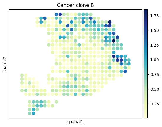
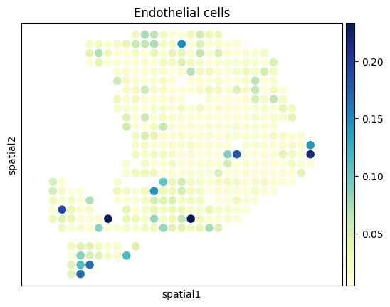
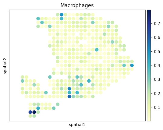
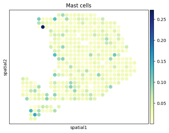
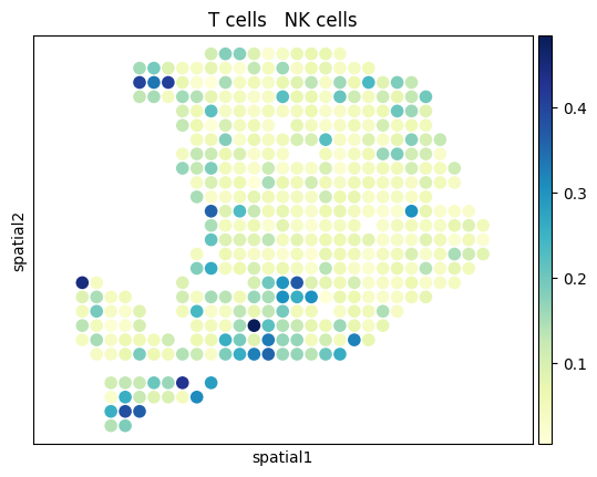
[27]:
from palettable.colorbrewer.sequential import YlGnBu_9
# to_plot_list = ['Acinar cells','Cancer clone A','Cancer clone B','Ductal']
to_plot_list = adata_sc.obs['CellType'].cat.categories
for to_plot in to_plot_list:
    ax = sc.pl.embedding(
        adata_st,
        basis='spatial',
        color=to_plot,
        show=False,
        color_map=YlGnBu_9.mpl_colormap
    )
    ax.axis('equal')