Reproducibility with original data

This tutorial demonstrates how to spatial data integration on Stereo-seq and Slide-seqV2 mouse olfactory bulb data using Pysodb and STAGATE based on pyG (PyTorch Geometric) framework.

A reference paper can be found at https://www.nature.com/articles/s41467-022-29439-6.

This tutorial refers to the following tutorial at https://stagate.readthedocs.io/en/latest/AT2.html. At the same time, the way of loadding data is modified by using Pysodb.

Import packages and set configurations

[1]:

# Use the Python warnings module to filter and ignore any warnings that may occur in the program after this point.
import warnings
warnings.filterwarnings("ignore")

[2]:

# Import several Python packages commonly used in data analysis and visualization:
# pandas (imported as pd) is a package for data manipulation and analysis
import pandas as pd
# numpy (imported as np) is a package for numerical computing with arrays
import numpy as np
# scanpy (imported as sc) is a package for single-cell RNA sequencing analysis
import scanpy as sc
import scanpy.external as sce
# matplotlib.pyplot (imported as plt) is a package for data visualization
import matplotlib.pyplot as plt
# Anndata is a package for working with annotated data.
import anndata as ad

[3]:

# Import a STAGATE_pyG module
import STAGATE_pyG as STAGATE

If users encounter the error “No module named ‘STAGATE_pyG’” when trying to import STAGATE_pyG package, first ensure that the “STAGATE_pyG” folder is located in the current script’s directory.

[4]:

# Imports a palettable package
import palettable
# Create two variables with lists of colors for categorical visualizations and biotechnology-related visualizations, respectively.
cmp_old = palettable.cartocolors.qualitative.Bold_10.mpl_colors
cmp_old_biotech = palettable.cartocolors.qualitative.Safe_4.mpl_colors

Streamline development of loading spatial data with Pysodb

[5]:

# Import pysodb package
# Pysodb is a Python package that provides a set of tools for working with SODB databases.
# SODB is a format used to store data in memory-mapped files for efficient access and querying.
# This package allows users to interact with SODB files using Python.
import pysodb

[6]:

# Initialization
sodb = pysodb.SODB()

load Slide-seqV2

[7]:

# Define names of dataset_name and experiment_name
dataset_name = 'stickels2020highly'
experiment_name = 'stickels2021highly_SlideSeqV2_Mouse_Olfactory_bulb_Puck_200127_15'
# Load a specific experiment
# It takes two arguments: the name of the dataset and the name of the experiment to load.
# Two arguments are available at https://gene.ai.tencent.com/SpatialOmics/.
adata = sodb.load_experiment(dataset_name,experiment_name)

load experiment[stickels2021highly_SlideSeqV2_Mouse_Olfactory_bulb_Puck_200127_15] in dataset[stickels2020highly]

[8]:

# The following three steps can be skipped, as the barcode information has already been added to the 'stickels2020highly' adata obtained through pysobd.
# Downloaded from https://drive.google.com/drive/folders/10lhz5VY7YfvHrtV40MwaqLmWz56U9eBP?usp=sharing
#used_barcode = pd.read_csv('data/used_barcodes.txt', sep='\t', header=None)
#used_barcode = used_barcode[0]

[9]:

#adata = adata[used_barcode,]

[10]:

# Filter genes to retain only those present in at least 50 cells
sc.pp.filter_genes(adata, min_cells=50)
print('After flitering: ', adata.shape)

After flitering:  (20139, 11750)

[11]:

adata

[11]:

AnnData object with n_obs × n_vars = 20139 × 11750
    obs: 'leiden'
    var: 'highly_variable', 'means', 'dispersions', 'dispersions_norm', 'n_cells'
    uns: 'hvg', 'leiden', 'leiden_colors', 'log1p', 'moranI', 'neighbors', 'pca', 'spatial_neighbors', 'umap'
    obsm: 'X_pca', 'X_umap', 'spatial'
    varm: 'PCs'
    obsp: 'connectivities', 'distances', 'spatial_connectivities', 'spatial_distances'

[12]:

# Create a dictionary named adata_list
adata_list = {}

[13]:

# Modify the names and save in the dictionary with the key 'SlideSeqV2'.
adata.obs_names = [x+'_SlideSeqV2' for x in adata.obs_names]
adata_list['SlideSeqV2'] = adata.copy()

load Stereo-seq

[14]:

# Define names of another dataset_name and experiment_name
dataset_name = 'Fu2021Unsupervised'
experiment_name = 'StereoSeq_MOB'
# Load another specific experiment
# It takes two arguments: the name of the dataset and the name of the experiment to load.
# Two arguments are available at https://gene.ai.tencent.com/SpatialOmics/.
adata = sodb.load_experiment(dataset_name,experiment_name)

load experiment[StereoSeq_MOB] in dataset[Fu2021Unsupervised]

[15]:

# Filter out genes
sc.pp.filter_genes(adata, min_cells=50)
print('After flitering: ', adata.shape)

After flitering:  (19109, 14376)

[16]:

# Update names and save in the dictionary under the key 'StereoSeq'
adata.obs_names = [x+'_StereoSeq' for x in adata.obs_names]
adata_list['StereoSeq'] = adata.copy()

Constructing the spatial network for each secion

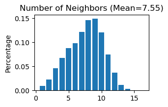
[17]:

# Use "STAGATE_pyG.Cal_Spatial_Net" to calculate a spatial graph with a radius cutoff of 50 for adata_list['SlideSeqV2']
STAGATE.Cal_Spatial_Net(adata_list['SlideSeqV2'], rad_cutoff=50)
# Use "STAGATE_pyG.Stats_Spatial_Net" to summarize cells and edges information for adata_list['SlideSeqV2']
STAGATE.Stats_Spatial_Net(adata_list['SlideSeqV2'])

------Calculating spatial graph...
The graph contains 228300 edges, 20139 cells.
11.3362 neighbors per cell on average.

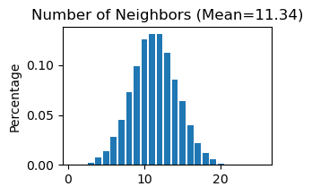
../_images/Spatial_data_integration_Reproducibility_with_original_data_24_1.png

[18]:

# Use "STAGATE_pyG.Cal_Spatial_Net" to calculate a spatial graph with a radius cutoff of 50 for adata_list['StereoSeq']
STAGATE.Cal_Spatial_Net(adata_list['StereoSeq'], rad_cutoff=50)
# Use "STAGATE_pyG.Stats_Spatial_Net" to summarize cells and edges information for adata_list['StereoSeq']
STAGATE.Stats_Spatial_Net(adata_list['StereoSeq'])

------Calculating spatial graph...
The graph contains 144318 edges, 19109 cells.
7.5524 neighbors per cell on average.

../_images/Spatial_data_integration_Reproducibility_with_original_data_25_1.png

[19]:

adata_list['SlideSeqV2'].uns['Spatial_Net']

[19]:

	Cell1	Cell2	Distance
0	AAAAAAACAAAAGG_SlideSeqV2	CTCCGGGCTCTTCA_SlideSeqV2	44.777226
1	AAAAAAACAAAAGG_SlideSeqV2	ATAAGTTGCCCCGT_SlideSeqV2	41.494698
2	AAAAAAACAAAAGG_SlideSeqV2	CCAGCAAAGCTACA_SlideSeqV2	29.429237
3	AAAAAAACAAAAGG_SlideSeqV2	CCTCCTTAACGTTA_SlideSeqV2	33.634060
4	AAAAAAACAAAAGG_SlideSeqV2	ACGTTCGCTCATAT_SlideSeqV2	15.307514
...	...	...	...
9	TTTTTTTTTTTTAT_SlideSeqV2	CTGACTTTAATCTA_SlideSeqV2	46.076567
10	TTTTTTTTTTTTAT_SlideSeqV2	CCTATAACAGCCTG_SlideSeqV2	30.802922
11	TTTTTTTTTTTTAT_SlideSeqV2	CTTGGGCATATAAG_SlideSeqV2	37.316216
12	TTTTTTTTTTTTAT_SlideSeqV2	CGGCAGGGATCCCT_SlideSeqV2	47.548291
13	TTTTTTTTTTTTAT_SlideSeqV2	TGGCAGGGATCCCT_SlideSeqV2	47.594643

228300 rows × 3 columns

[20]:

# Concatenate 'SlideSeqV2' and 'StereoSeq' into a single AnnData object named 'adata'
adata = sc.concat([adata_list['SlideSeqV2'], adata_list['StereoSeq']], keys=None)

[21]:

# Concatenate two 'Spatial_Net'
adata.uns['Spatial_Net'] = pd.concat([adata_list['SlideSeqV2'].uns['Spatial_Net'], adata_list['StereoSeq'].uns['Spatial_Net']])

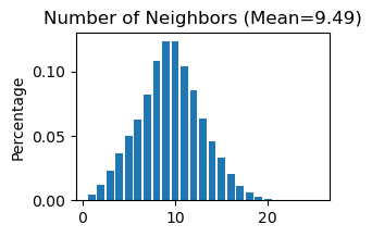
[22]:

# Use "STAGATE_pyG.Stats_Spatial_Net" to summarize cells and edges information for whole adata
STAGATE.Stats_Spatial_Net(adata)

../_images/Spatial_data_integration_Reproducibility_with_original_data_29_0.png

[23]:

# Normalization
sc.pp.highly_variable_genes(adata, flavor="seurat_v3", n_top_genes=3000)
sc.pp.normalize_total(adata, target_sum=1e4)
sc.pp.log1p(adata)

[24]:

adata

[24]:

AnnData object with n_obs × n_vars = 39248 × 10782
    obs: 'leiden'
    var: 'highly_variable', 'highly_variable_rank', 'means', 'variances', 'variances_norm'
    uns: 'Spatial_Net', 'hvg', 'log1p'
    obsm: 'X_pca', 'X_umap', 'spatial'

Running STAGATE

[25]:

adata = STAGATE.train_STAGATE(adata, n_epochs=500, device='cpu')

Size of Input:  (39248, 3000)

100%|██████████| 500/500 [1:41:41<00:00, 12.20s/it]

Spatial Clustering

[26]:

# Create a new column 'Tech' by splitting each name and selecting the last element
adata.obs['Tech'] = [x.split('_')[-1] for x in adata.obs_names]

[27]:

# Calculates neighbors in the 'STAGATE' representation, applies UMAP, and performs louvain clustering
sc.pp.neighbors(adata, use_rep='STAGATE')
sc.tl.umap(adata)
sc.tl.louvain(adata,resolution=0.3)

When encountering the Error “No module named ‘igraph’”, users should activate the virtual environment at the terminal and execute “pip install igraph”.

When encountering the Error “No module named ‘louvain’”, users should activate the virtual environment at the terminal and execute “pip install louvain”.

[28]:

# Plot a UMAP projection
plt.rcParams["figure.figsize"] = (3, 3)
sc.pl.umap(adata, color='Tech', title='Unintegrated',show=False,palette=cmp_old_biotech)
#plt.savefig('figures/old_before_umap.png',dpi=400,transparent=True,bbox_inches='tight')
#plt.savefig('figures/old_before_umap.pdf',dpi=400,transparent=True,bbox_inches='tight')

[28]:

<Axes: title={'center': 'Unintegrated'}, xlabel='UMAP1', ylabel='UMAP2'>

../_images/Spatial_data_integration_Reproducibility_with_original_data_38_1.png

[29]:

# Generate a plot of the UMAP embedding colored by louvain
plt.rcParams["figure.figsize"] = (3, 3)
sc.pl.umap(adata, color='louvain',show=False,palette=cmp_old)
#plt.savefig('figures/old_before_umap_leiden.png',dpi=400,transparent=True,bbox_inches='tight')
#plt.savefig('figures/old_before_umap_leiden.pdf',dpi=400,transparent=True,bbox_inches='tight')

[29]:

<Axes: title={'center': 'louvain'}, xlabel='UMAP1', ylabel='UMAP2'>

../_images/Spatial_data_integration_Reproducibility_with_original_data_39_1.png

[30]:

# Display spatial distribution of cells colored by louvain clustering for two sequencing technologies ('StereoSeq' and 'SlideSeqV2')
fig, axs = plt.subplots(1, 2, figsize=(6, 3))
it=0
for temp_tech in ['StereoSeq', 'SlideSeqV2']:
    temp_adata = adata[adata.obs['Tech']==temp_tech, ]
    if it == 1:
        sc.pl.embedding(temp_adata, basis="spatial", color="louvain",s=6, ax=axs[it],
                        show=False, title=temp_tech)
    else:
        sc.pl.embedding(temp_adata, basis="spatial", color="louvain",s=6, ax=axs[it], legend_loc=None,
                        show=False, title=temp_tech)
    it+=1
#plt.savefig('figures/old_before_spatial_leiden0.3.png',dpi=400,transparent=True,bbox_inches='tight')
#plt.savefig('figures/old_before_spatial_leiden0.3.pdf',dpi=400,transparent=True,bbox_inches='tight')

../_images/Spatial_data_integration_Reproducibility_with_original_data_40_0.png

Perform Harmony for spatial data intergration

Harmony is an algorithm for integrating multiple high-dimensional datasets It can be employed as a reference at https://github.com/slowkow/harmonypy and https://pypi.org/project/harmonypy/

[31]:

# Import harmonypy package
import harmonypy as hm

[32]:

# Use STAGATE representation to create 'meta_data' for harmony
data_mat = adata.obsm['STAGATE'].copy()
meta_data = adata.obs.copy()

[33]:

# Run harmony for STAGATE representation
ho = hm.run_harmony(data_mat, meta_data, ['Tech'])

2023-04-03 11:20:28,820 - harmonypy - INFO - Computing initial centroids with sklearn.KMeans...
2023-04-03 11:20:34,852 - harmonypy - INFO - sklearn.KMeans initialization complete.
2023-04-03 11:20:34,995 - harmonypy - INFO - Iteration 1 of 10
2023-04-03 11:20:42,857 - harmonypy - INFO - Iteration 2 of 10
2023-04-03 11:20:50,987 - harmonypy - INFO - Iteration 3 of 10
2023-04-03 11:20:58,029 - harmonypy - INFO - Converged after 3 iterations

[34]:

# Write the adjusted PCs to a new file.
res = pd.DataFrame(ho.Z_corr)
res.columns = adata.obs_names

[35]:

# Creates a new AnnData object adata_Harmony using a transpose of the res matrix
adata_Harmony = sc.AnnData(res.T)

[36]:

adata_Harmony.obsm['spatial'] = pd.DataFrame(adata.obsm['spatial'], index=adata.obs_names).loc[adata_Harmony.obs_names,].values
adata_Harmony.obs['Tech'] = adata.obs.loc[adata_Harmony.obs_names, 'Tech']

Spatial Clustering after integration

[37]:

# Calculate neighbors, apply UMAP, and perform louvain clustering for the integrated data
sc.pp.neighbors(adata_Harmony)
sc.tl.umap(adata_Harmony)
sc.tl.louvain(adata_Harmony, resolution=0.3)

[38]:

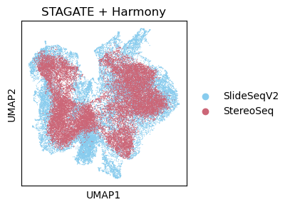
# Plot a UMAP embedding colored by louvain after integration
plt.rcParams["figure.figsize"] = (3, 3)
sc.pl.umap(adata_Harmony, color='Tech', title='STAGATE + Harmony',show=False,palette=cmp_old_biotech)
#plt.savefig('figures/old_after_umap.png',dpi=400,transparent=True,bbox_inches='tight')
#plt.savefig('figures/old_after_umap.pdf',dpi=400,transparent=True,bbox_inches='tight')

[38]:

<Axes: title={'center': 'STAGATE + Harmony'}, xlabel='UMAP1', ylabel='UMAP2'>

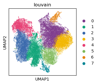
../_images/Spatial_data_integration_Reproducibility_with_original_data_51_1.png

[39]:

# Display spatial distribution of cells colored by louvain clustering for two sequencing technologies ('StereoSeq' and 'SlideSeqV2') after integration
plt.rcParams["figure.figsize"] = (3, 3)
sc.pl.umap(adata_Harmony, color='louvain',show=False,palette=cmp_old)
#plt.savefig('figures/old_after_umap_leiden0.4.png',dpi=400,transparent=True,bbox_inches='tight')
#plt.savefig('figures/old_after_umap_leiden0.4.pdf',dpi=400,transparent=True,bbox_inches='tight')

[39]:

<Axes: title={'center': 'louvain'}, xlabel='UMAP1', ylabel='UMAP2'>

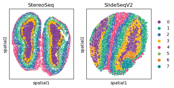
../_images/Spatial_data_integration_Reproducibility_with_original_data_52_1.png

[40]:

# Display spatial distribution of cells colored by louvain clustering for two sequencing technologies ('StereoSeq' and 'SlideSeqV2') after integration
fig, axs = plt.subplots(1, 2, figsize=(6, 3))
it=0
for temp_tech in ['StereoSeq', 'SlideSeqV2']:
    temp_adata = adata_Harmony[adata_Harmony.obs['Tech']==temp_tech, ]
    if it == 1:
        sc.pl.embedding(temp_adata, basis="spatial", color="louvain",s=6, ax=axs[it],
                        show=False, title=temp_tech)
    else:
        sc.pl.embedding(temp_adata, basis="spatial", color="louvain",s=6, ax=axs[it], legend_loc=None,
                        show=False, title=temp_tech)
    it+=1
#plt.savefig('figures/old_after_spatial_leiden0.4.png',dpi=400,transparent=True,bbox_inches='tight')
#plt.savefig('figures/old_after_spatial_leiden0.4.pdf',dpi=400,transparent=True,bbox_inches='tight')

../_images/Spatial_data_integration_Reproducibility_with_original_data_53_0.png