Reproducibility with original data (DLPFC)

This tutorial demonstrates how to pseudo-spatiotemporal analysis on 10X Visium human dorsolateral prefrontal cortex data using Pysodb and SpaceFlow.

A reference paper can be found at https://www.nature.com/articles/s41467-022-31739-w.

This tutorial refers to the following tutorial at https://github.com/hongleir/SpaceFlow/blob/master/tutorials/seqfish_mouse_embryogenesis.ipynb. At the same time, the way of loadding data is modified by using Pysodb.

Import packages and set configurations

[1]:

# Use the Python warnings module to filter and ignore any warnings that may occur in the program after this point.
import warnings
warnings.filterwarnings("ignore")

[2]:

# Import several python packages commonly used in data analysis and visualization.
# numpy (imported as np) is a package for numerical computing with arrays.
import numpy as np
# scanpy (imported as sc) is a package for single-cell RNA sequencing analysis.
import scanpy as sc
# matplotlib.pyplot (imported as plt) is a package for data visualization.
import matplotlib.pyplot as plt

[3]:

# from SpaceFlow package import SpaceFlow module
from SpaceFlow import SpaceFlow

[4]:

# Imports a palettable package
import palettable
# Create three variables with lists of colors for categorical visualizations and biotechnology-related visualizations, respectively.
cmp_pspace = palettable.cartocolors.diverging.TealRose_7.mpl_colormap
cmp_domain = palettable.cartocolors.qualitative.Pastel_10.mpl_colors
cmp_ct = palettable.cartocolors.qualitative.Safe_10.mpl_colors

When encountering the error “No module name ‘palettable’”, users need to activate conda’s virtual environment first at the terminal and run the following command in the terminal: “pip install palettable”. This approach can be applied to other packages as well, by replacing ‘palettable’ with the name of the desired package.

Streamline development of loading spatial data with Pysodb

[5]:

# Import pysodb package
# Pysodb is a Python package that provides a set of tools for working with SODB databases.
# SODB is a format used to store data in memory-mapped files for efficient access and querying.
# This package allows users to interact with SODB files using Python.
import pysodb

[6]:

# Initialize the sodb object
sodb = pysodb.SODB()

[7]:

# Define names of the dataset_name and experiment_name
dataset_name = 'maynard2021trans'
experiment_name = '151671'
# Load a specific experiment
# It takes two arguments: the name of the dataset and the name of the experiment to load.
# Two arguments are available at https://gene.ai.tencent.com/SpatialOmics/.
#%%time
adata = sodb.load_experiment(dataset_name,experiment_name)

load experiment[151671] in dataset[maynard2021trans]

Perform SpaceFlow for pseudo-spatiotemporal analysis

[8]:

# Create SpaceFlow Object
#%%time
sf = SpaceFlow.SpaceFlow(
    count_matrix=adata.X,
    spatial_locs=adata.obsm['spatial'],
    sample_names=adata.obs_names,
    gene_names=adata.var_names
)

When encountering the error “Error: The truth value of an array with more than one element is ambiguous. Use a.any() or a.all().”, in the “SpaceFlow.py” file from the SpaceFlow package, the user is advised to make the following modifications within the init function. Replace “elif count_matrix and spatial_locs:” with “elif count_matrix is not None and spatial_locs is not None:”. Additionally, modify “if gene_names:” and “if sample_names:” to “if gene_names is not None:” and “if sample_names is not None:” respectively. The above modifications ensure that the if statement returns a single boolean value. respectively.

[9]:

adata

[9]:

AnnData object with n_obs × n_vars = 4110 × 33538
    obs: 'in_tissue', 'array_row', 'array_col', 'Region', 'leiden'
    var: 'gene_ids', 'feature_types', 'genome', 'highly_variable', 'means', 'dispersions', 'dispersions_norm'
    uns: 'hvg', 'leiden', 'leiden_colors', 'log1p', 'moranI', 'neighbors', 'pca', 'spatial', 'spatial_neighbors', 'umap'
    obsm: 'X_pca', 'X_umap', 'spatial'
    varm: 'PCs'
    obsp: 'connectivities', 'distances', 'spatial_connectivities', 'spatial_distances'

[10]:

# Preprocess data
#%%time
sf.preprocessing_data(n_top_genes=3000)

When encountering the error “Error: You can drop duplicate edges by setting the ‘duplicates’ kwarg”,in “SpaceFlow.py” from the SpaceFlow package, modify the preprocessing_data function by: (1) removing target_sum=1e4 from sc.pp.normalize_total(); (2) changing the flavor argument to ‘seurat’ in sc.pp.highly_variable_genes(); (3) Save and rerun the analysis.

When encountering the error “Error: module ‘networkx’ has no attribute ‘to_scipy_sparse_matrix’”, users should first activate the virtual environment at the terminal and then downgrade NetworkX with the following command：”pip install networkx==2.8”. This will ensure that the correct version of NetworkX is installed within the specified virtual environment.

[11]:

# Train a deep graph network model
#%%time
sf.train(
    spatial_regularization_strength=0.1,
    z_dim=50,
    lr=1e-3,
    epochs=1000,
    max_patience=50,
    min_stop=100,
    random_seed=42,
    gpu=0,
    regularization_acceleration=True,
    edge_subset_sz=1000000
)

Epoch 2/1000, Loss: 1.6001609563827515
Epoch 12/1000, Loss: 1.4461232423782349
Epoch 22/1000, Loss: 1.4314894676208496
Epoch 32/1000, Loss: 1.4025373458862305
Epoch 42/1000, Loss: 1.3406403064727783
Epoch 52/1000, Loss: 1.202500820159912
Epoch 62/1000, Loss: 0.9297404289245605
Epoch 72/1000, Loss: 0.6375124454498291
Epoch 82/1000, Loss: 0.4029056429862976
Epoch 92/1000, Loss: 0.2597547173500061
Epoch 102/1000, Loss: 0.17297157645225525
Epoch 112/1000, Loss: 0.12740349769592285
Epoch 122/1000, Loss: 0.10466508567333221
Epoch 132/1000, Loss: 0.08336742222309113
Epoch 142/1000, Loss: 0.07964801788330078
Epoch 152/1000, Loss: 0.07678414136171341
Epoch 162/1000, Loss: 0.069277323782444
Epoch 172/1000, Loss: 0.0713764876127243
Epoch 182/1000, Loss: 0.06293175369501114
Epoch 192/1000, Loss: 0.06099879369139671
Epoch 202/1000, Loss: 0.061921969056129456
Epoch 212/1000, Loss: 0.05519292131066322
Epoch 222/1000, Loss: 0.06154436245560646
Epoch 232/1000, Loss: 0.05294334143400192
Epoch 242/1000, Loss: 0.047114331275224686
Epoch 252/1000, Loss: 0.051006168127059937
Epoch 262/1000, Loss: 0.04537639394402504
Epoch 272/1000, Loss: 0.05118394270539284
Epoch 282/1000, Loss: 0.050518788397312164
Epoch 292/1000, Loss: 0.045374199748039246
Epoch 302/1000, Loss: 0.04892214760184288
Epoch 312/1000, Loss: 0.04162988066673279
Epoch 322/1000, Loss: 0.04166189581155777
Epoch 332/1000, Loss: 0.043898724019527435
Epoch 342/1000, Loss: 0.04035808518528938
Epoch 352/1000, Loss: 0.04706918075680733
Epoch 362/1000, Loss: 0.04220199957489967
Epoch 372/1000, Loss: 0.03935319185256958
Epoch 382/1000, Loss: 0.050716839730739594
Epoch 392/1000, Loss: 0.0474902018904686
Epoch 402/1000, Loss: 0.041612617671489716
Epoch 412/1000, Loss: 0.0376250222325325
Epoch 422/1000, Loss: 0.03883547708392143
Epoch 432/1000, Loss: 0.03730320930480957
Epoch 442/1000, Loss: 0.03816107660531998
Epoch 452/1000, Loss: 0.03693684563040733
Epoch 462/1000, Loss: 0.03563809394836426
Epoch 472/1000, Loss: 0.038218624889850616
Epoch 482/1000, Loss: 0.042877957224845886
Epoch 492/1000, Loss: 0.035798318684101105
Epoch 502/1000, Loss: 0.045439526438713074
Epoch 512/1000, Loss: 0.04299004375934601
Epoch 522/1000, Loss: 0.0379679910838604
Epoch 532/1000, Loss: 0.03415396809577942
Epoch 542/1000, Loss: 0.03743215650320053
Epoch 552/1000, Loss: 0.039857201278209686
Epoch 562/1000, Loss: 0.03960778936743736
Epoch 572/1000, Loss: 0.04264502972364426
Epoch 582/1000, Loss: 0.03573727235198021
Epoch 592/1000, Loss: 0.03262363746762276
Epoch 602/1000, Loss: 0.0346861407160759
Epoch 612/1000, Loss: 0.03681035339832306
Epoch 622/1000, Loss: 0.048560068011283875
Epoch 632/1000, Loss: 0.03910374641418457
Epoch 642/1000, Loss: 0.03717295080423355
Epoch 652/1000, Loss: 0.032764457166194916
Epoch 662/1000, Loss: 0.035095784813165665
Epoch 672/1000, Loss: 0.030956480652093887
Epoch 682/1000, Loss: 0.033467892557382584
Epoch 692/1000, Loss: 0.033409349620342255
Epoch 702/1000, Loss: 0.030765127390623093
Epoch 712/1000, Loss: 0.030486250296235085
Epoch 722/1000, Loss: 0.03218876197934151
Epoch 732/1000, Loss: 0.03625836223363876
Epoch 742/1000, Loss: 0.031791478395462036
Epoch 752/1000, Loss: 0.03017842024564743
Epoch 762/1000, Loss: 0.02982253022491932
Epoch 772/1000, Loss: 0.02927223965525627
Epoch 782/1000, Loss: 0.036921072751283646
Epoch 792/1000, Loss: 0.036078497767448425
Epoch 802/1000, Loss: 0.031135806813836098
Epoch 812/1000, Loss: 0.031050482764840126
Epoch 822/1000, Loss: 0.046886757016181946
Epoch 832/1000, Loss: 0.029026398435235023
Epoch 842/1000, Loss: 0.03208329528570175
Epoch 852/1000, Loss: 0.029403438791632652
Training complete!
Embedding is saved at ./embedding.tsv

[11]:

array([[ 1.7401947e+00,  2.8369801e+00,  2.2377011e-01, ...,
         3.7823334e-01, -3.9555269e-01, -5.8662368e-04],
       [ 2.1318159e+00,  1.6539254e+00, -2.3631152e-02, ...,
         1.1321043e+00, -4.1971338e-01,  1.5606171e+00],
       [ 1.8066632e+00,  2.2979531e+00, -6.5132994e-03, ...,
         2.5315709e-02, -4.6509734e-01, -5.6492598e-03],
       ...,
       [ 1.7791069e+00,  2.6776686e+00, -2.0510532e-02, ...,
         7.8728390e-01, -3.9734748e-01,  1.3013610e+00],
       [ 1.5107570e+00,  2.0946822e+00,  1.1377124e+00, ...,
         8.1175212e-03, -5.2531648e-01,  9.9224053e-02],
       [ 1.4871329e+00,  1.9591911e+00, -3.1830516e-02, ...,
         8.9999894e-03, -3.4401137e-01, -1.1019838e-03]], dtype=float32)

[12]:

# Idenfify the spatiotemporal patterns through pseudo-Spatiotemporal Map (pSM)
sf.pseudo_Spatiotemporal_Map(pSM_values_save_filepath="./pSM_values.tsv", n_neighbors=20, resolution=1.0)

Performing pseudo-Spatiotemporal Map
pseudo-Spatiotemporal Map(pSM) calculation complete, pSM values of cells or spots saved at ./pSM_values.tsv!

[13]:

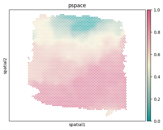
# Create a new column called 'pspace' from pSM values of cells or spots.
adata.obs['pspace'] = sf.pSM_values

[14]:

# Visualize spatial coordinates in a scatterplot colored by pspace
ax = sc.pl.embedding(adata,basis='spatial',color='pspace',show=False,color_map=cmp_pspace)
ax.axis('equal')
#plt.savefig('figures/DLPFC_pspace.png',bbox_inches='tight',transparent=True,dpi=400)
#plt.savefig('figures/DLPFC_pspace.pdf',bbox_inches='tight',transparent=True,dpi=400)

[14]:

(2755.35, 12383.65, 2191.15, 12197.85)

../_images/Pseudo-spatiotemporal_analysis_Reproducibility_with_original_data_%28DLPFC%29_21_1.png

[15]:

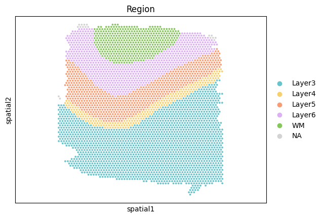
# Visualize spatial coordinates in a scatterplot colored by Region
ax = sc.pl.embedding(adata,basis='spatial',color='Region',show=False,palette=cmp_domain)
ax.axis('equal')
#plt.savefig('figures/seqFISH_ct.png',bbox_inches='tight',transparent=True,dpi=400)
#plt.savefig('figures/seqFISH_ct.pdf',bbox_inches='tight',transparent=True,dpi=400)

[15]:

(2755.35, 12383.65, 2191.15, 12197.85)

../_images/Pseudo-spatiotemporal_analysis_Reproducibility_with_original_data_%28DLPFC%29_22_1.png