Application with new data

This tutorial demonstrates how to pseudo-spatiotemporal analysis on BaristaSeq mouse visual cortex data using Pysodb and SpaceFlow.

A reference paper can be found at https://www.nature.com/articles/s41467-022-31739-w.

This tutorial refers to the following tutorial at https://github.com/hongleir/SpaceFlow/blob/master/tutorials/seqfish_mouse_embryogenesis.ipynb. At the same time, the way of loadding data is modified by using Pysodb.

Import packages and set configurations

[1]:

# Use the Python warnings module to filter and ignore any warnings that may occur in the program after this point.
import warnings
warnings.filterwarnings("ignore")

[2]:

# Import several python packages commonly used in data analysis and visualization.
# numpy (imported as np) is a package for numerical computing with arrays.
import numpy as np
# scanpy (imported as sc) is a package for single-cell RNA sequencing analysis.
import scanpy as sc
# matplotlib.pyplot (imported as plt) is a package for data visualization.
import matplotlib.pyplot as plt
# seaborn (imported as sns) is a package for statistical data visualization, providing high-level interfaces for creating informative and attractive visualizations.
import seaborn as sns

[3]:

# from SpaceFlow package import SpaceFlow module
from SpaceFlow import SpaceFlow

[4]:

# Imports a palettable package
import palettable
# Create three variables with lists of colors for categorical visualizations and biotechnology-related visualizations, respectively.
cmp_pspace = palettable.cartocolors.diverging.TealRose_7.mpl_colormap
cmp_domain = palettable.cartocolors.qualitative.Pastel_10.mpl_colors
cmp_ct = palettable.cartocolors.qualitative.Safe_10.mpl_colors

When encountering the error “No module name ‘palettable’”, users need to activate conda’s virtual environment first at the terminal and run the following command in the terminal: “pip install palettable”. This approach can be applied to other packages as well, by replacing ‘palettable’ with the name of the desired package.

Streamline development of loading spatial data with Pysodb

[5]:

# Import pysodb package
# Pysodb is a Python package that provides a set of tools for working with SODB databases.
# SODB is a format used to store data in memory-mapped files for efficient access and querying.
# This package allows users to interact with SODB files using Python.
import pysodb

[6]:

# Initialize the sodb object
sodb = pysodb.SODB()

[7]:

# Define names of the dataset_name and experiment_name
dataset_name = 'Sun2021Integrating'
experiment_name = 'Slice_1'
# Load a specific experiment
# It takes two arguments: the name of the dataset and the name of the experiment to load.
# Two arguments are available at https://gene.ai.tencent.com/SpatialOmics/.
#%%time
adata = sodb.load_experiment(dataset_name,experiment_name)

load experiment[Slice_1] in dataset[Sun2021Integrating]

[8]:

# Remove cells belong to the layers 'outside_VISp' and 'VISp'
adata = adata[adata.obs['layer']!='outside_VISp']
adata = adata[adata.obs['layer']!='VISp']

[9]:

# Filter out genes
sc.pp.filter_genes(adata, min_cells=3)

Perform SpaceFlow for pseudo-spatiotemporal analysis

[10]:

# Create SpaceFlow Object
#%%time
#sf = SpaceFlow.SpaceFlow(adata=adata)
sf = SpaceFlow.SpaceFlow(
    count_matrix=adata.X,
    spatial_locs=adata.obsm['spatial'],
    sample_names=adata.obs_names,
    gene_names=adata.var_names
)

When encountering the error “Error: The truth value of an array with more than one element is ambiguous. Use a.any() or a.all().”, in the “SpaceFlow.py” file from the SpaceFlow package, the user is advised to make the following modifications within the init function. Replace “elif count_matrix and spatial_locs:” with “elif count_matrix is not None and spatial_locs is not None:”. Additionally, modify “if gene_names:” and “if sample_names:” to “if gene_names is not None:” and “if sample_names is not None:” respectively. The above modifications ensure that the if statement returns a single boolean value. respectively.

[11]:

# Preprocess data
#%%time
sf.preprocessing_data(n_top_genes=3000)

When encountering the error “Error: You can drop duplicate edges by setting the ‘duplicates’ kwarg”,in “SpaceFlow.py” from the SpaceFlow package, modify the preprocessing_data function by: (1) removing target_sum=1e4 from sc.pp.normalize_total(); (2) changing the flavor argument to ‘seurat’ in sc.pp.highly_variable_genes(); (3) Save and rerun the analysis.

When encountering the error “Error: module ‘networkx’ has no attribute ‘to_scipy_sparse_matrix’”, users should first activate the virtual environment at the terminal and then downgrade NetworkX with the following command：”pip install networkx==2.8”. This will ensure that the correct version of NetworkX is installed within the specified virtual environment.

[12]:

# Train a deep graph network model
#%%time
sf.train(
    spatial_regularization_strength=0.1,
    z_dim=50,
    lr=1e-3,
    epochs=1000,
    max_patience=50,
    min_stop=100,
    random_seed=42,
    gpu=0,
    regularization_acceleration=True,
    edge_subset_sz=1000000
)

Epoch 2/1000, Loss: 1.4427732229232788
Epoch 12/1000, Loss: 1.404854416847229
Epoch 22/1000, Loss: 1.355185866355896
Epoch 32/1000, Loss: 1.278242826461792
Epoch 42/1000, Loss: 1.1435610055923462
Epoch 52/1000, Loss: 0.9432040452957153
Epoch 62/1000, Loss: 0.714905321598053
Epoch 72/1000, Loss: 0.5822354555130005
Epoch 82/1000, Loss: 0.5121979713439941
Epoch 92/1000, Loss: 0.425785630941391
Epoch 102/1000, Loss: 0.37741926312446594
Epoch 112/1000, Loss: 0.3343759775161743
Epoch 122/1000, Loss: 0.3119865655899048
Epoch 132/1000, Loss: 0.26779788732528687
Epoch 142/1000, Loss: 0.22297403216362
Epoch 152/1000, Loss: 0.28504329919815063
Epoch 162/1000, Loss: 0.22740697860717773
Epoch 172/1000, Loss: 0.234877809882164
Epoch 182/1000, Loss: 0.1949552297592163
Epoch 192/1000, Loss: 0.20016708970069885
Epoch 202/1000, Loss: 0.2028239667415619
Epoch 212/1000, Loss: 0.173057422041893
Epoch 222/1000, Loss: 0.21973812580108643
Epoch 232/1000, Loss: 0.17184185981750488
Epoch 242/1000, Loss: 0.2074703425168991
Epoch 252/1000, Loss: 0.19310833513736725
Epoch 262/1000, Loss: 0.2128731906414032
Epoch 272/1000, Loss: 0.17560149729251862
Epoch 282/1000, Loss: 0.2080163210630417
Epoch 292/1000, Loss: 0.18244342505931854
Epoch 302/1000, Loss: 0.17130610346794128
Epoch 312/1000, Loss: 0.16225826740264893
Epoch 322/1000, Loss: 0.15506717562675476
Epoch 332/1000, Loss: 0.1312013417482376
Epoch 342/1000, Loss: 0.14738863706588745
Epoch 352/1000, Loss: 0.1790708303451538
Epoch 362/1000, Loss: 0.1254740208387375
Epoch 372/1000, Loss: 0.1862727850675583
Epoch 382/1000, Loss: 0.17113451659679413
Epoch 392/1000, Loss: 0.141239196062088
Epoch 402/1000, Loss: 0.11042129248380661
Epoch 412/1000, Loss: 0.1695185899734497
Epoch 422/1000, Loss: 0.11782366037368774
Epoch 432/1000, Loss: 0.14781805872917175
Epoch 442/1000, Loss: 0.17524565756320953
Epoch 452/1000, Loss: 0.13630664348602295
Epoch 462/1000, Loss: 0.15702477097511292
Epoch 472/1000, Loss: 0.11048941314220428
Epoch 482/1000, Loss: 0.12970110774040222
Epoch 492/1000, Loss: 0.15136636793613434
Epoch 502/1000, Loss: 0.10564137995243073
Epoch 512/1000, Loss: 0.14658908545970917
Epoch 522/1000, Loss: 0.11960890889167786
Epoch 532/1000, Loss: 0.13005761802196503
Epoch 542/1000, Loss: 0.11053520441055298
Epoch 552/1000, Loss: 0.11907373368740082
Epoch 562/1000, Loss: 0.1232338398694992
Epoch 572/1000, Loss: 0.11129128932952881
Epoch 582/1000, Loss: 0.10171715170145035
Epoch 592/1000, Loss: 0.09877597540616989
Epoch 602/1000, Loss: 0.12555311620235443
Epoch 612/1000, Loss: 0.10553622245788574
Epoch 622/1000, Loss: 0.13101576268672943
Epoch 632/1000, Loss: 0.1205601841211319
Training complete!
Embedding is saved at ./embedding.tsv

[12]:

array([[ 0.8899192 ,  0.01435345,  0.7866027 , ...,  0.5507234 ,
        -0.03758647, -0.08572218],
       [ 0.8003285 ,  0.00401396,  0.72124624, ...,  0.42994535,
        -0.04228881, -0.06209074],
       [ 0.8963664 ,  0.01202957,  0.7585074 , ...,  0.59778905,
        -0.03772109, -0.08880965],
       ...,
       [ 0.48202616,  0.01098088,  0.6471445 , ..., -0.00690297,
         0.73529345,  0.32098433],
       [ 0.5201945 ,  0.00505677,  0.6052369 , ..., -0.00182656,
         0.46181548,  0.19144082],
       [ 0.4544619 ,  0.00249925,  0.5253095 , ..., -0.00313081,
         0.6240246 ,  0.4014499 ]], dtype=float32)

[13]:

# Idenfify the spatiotemporal patterns through pseudo-Spatiotemporal Map (pSM)
sf.pseudo_Spatiotemporal_Map(pSM_values_save_filepath="./pSM_values.tsv", n_neighbors=20, resolution=1.0)

Performing pseudo-Spatiotemporal Map
pseudo-Spatiotemporal Map(pSM) calculation complete, pSM values of cells or spots saved at ./pSM_values.tsv!

[14]:

# Create a new column called 'pspace' from pSM values
adata.obs['pspace'] = np.array(sf.pSM_values)

[15]:

# Create a UMAP projection from SpaceFlow's embedding
adata.obsm['embedding'] = sf.embedding
sc.pp.neighbors(adata, n_neighbors=20, use_rep='embedding')
sc.tl.umap(adata)

[16]:

# Since this dataset contains 'depth_um' in obs, a iroot was set to be the cell with smallest depth_um.
# For datasets without depth information, one can use the pseudo_Spatiotemporal_Map function
# Here set the iroot according to "depth_um"

# Select the root cell for trajectory inference based on its depth, by setting the index of the cell with the smallest 'depth_um' value as the root
adata.uns['iroot'] = np.argmin(adata.obs['depth_um'])
sc.tl.diffmap(adata)
sc.tl.dpt(adata)

[17]:

# Plot spatial embedding and UMAP embedding for diffusion pseudotime and layer(label), respectively

# si = 'Slice_1'

ax = sc.pl.embedding(adata,basis='spatial',color=['dpt_pseudotime'],show=False,color_map=cmp_pspace)
ax.axis('equal')
# plt.savefig(f'../figures/pspace/BaristaSeq_{si}_pspace.png',bbox_inches='tight',transparent=True,dpi=400)
# plt.savefig(f'../figures/pspace/BaristaSeq_{si}_pspace.pdf',bbox_inches='tight',transparent=True,dpi=400)

ax = sc.pl.embedding(adata,basis='spatial',color='layer',show=False,palette=cmp_domain)
ax.axis('equal')
# plt.savefig(f'../figures/pspace/BaristaSeq_{si}_domain.png',bbox_inches='tight',transparent=True,dpi=400)
# plt.savefig(f'../figures/pspace/BaristaSeq_{si}_domain.pdf',bbox_inches='tight',transparent=True,dpi=400)

fig, ax = plt.subplots()
fig.set_size_inches(4, 4)
sc.pl.embedding(adata,basis='X_umap',color='layer',show=False,palette=cmp_domain,ax=ax)
#ax.axis('equal')
# plt.savefig(f'../figures/pspace/BaristaSeq_{si}_UMAP_domain.png',bbox_inches='tight',transparent=True,dpi=400)
# plt.savefig(f'../figures/pspace/BaristaSeq_{si}_UMAP_domain.pdf',bbox_inches='tight',transparent=True,dpi=400)

fig, ax = plt.subplots()
fig.set_size_inches(4, 4)
sc.pl.embedding(adata,basis='X_umap',color=['dpt_pseudotime'],show=False,color_map=cmp_pspace,ax=ax)
#ax.axis('equal')
# plt.savefig(f'../figures/pspace/BaristaSeq_{si}_UMAP_pspace.png',bbox_inches='tight',transparent=True,dpi=400)
# plt.savefig(f'../figures/pspace/BaristaSeq_{si}_UMAP_pspace.pdf',bbox_inches='tight',transparent=True,dpi=400)

[17]:

<Axes: title={'center': 'dpt_pseudotime'}, xlabel='X_umap1', ylabel='X_umap2'>

../_images/Pseudo-spatiotemporal_analysis_Application_with_new_data_24_1.png

../_images/Pseudo-spatiotemporal_analysis_Application_with_new_data_24_2.png

../_images/Pseudo-spatiotemporal_analysis_Application_with_new_data_24_3.png

../_images/Pseudo-spatiotemporal_analysis_Application_with_new_data_24_4.png

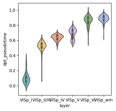
[18]:

# Check whether the pseudo-spatiotemporal (dpt_pseudotime) value from infer increases according to the layer of the cortex
adata_use = adata
fig,ax = plt.subplots(figsize=(4,4))
sns.violinplot(data=adata_use.obs,x='layer',y='dpt_pseudotime',palette = adata_use.uns['layer_colors'],ax=ax)
# plt.savefig(f'../figures/pspace/BaristaSeq_{si}_violin.png',bbox_inches='tight',transparent=True,dpi=400)
# plt.savefig(f'../figures/pspace/BaristaSeq_{si}_violin.pdf',bbox_inches='tight',transparent=True,dpi=400)

[18]:

<Axes: xlabel='layer', ylabel='dpt_pseudotime'>

../_images/Pseudo-spatiotemporal_analysis_Application_with_new_data_25_1.png

[19]:

adata.obs

[19]:

	Slice	x	y	Dist to pia	Dist to bottom	Angle	unused-1	unused-2	x_um	y_um	depth_um	layer	leiden	pspace	dpt_pseudotime
20022	1	12186.20	8617.70	1029.630	205.270	174.894	0	0	1218.620	861.770	1093.752193	VISp_VI	1	0.911279	0.903298
20023	1	12789.10	8690.82	1072.540	168.011	172.700	0	0	1278.910	869.082	1139.629730	VISp_VI	4	0.892462	0.882942
20024	1	11927.80	8715.20	1003.280	231.018	177.522	0	0	1192.780	871.520	1066.880345	VISp_VI	1	0.928142	0.921913
20025	1	12860.60	8729.82	1075.760	165.770	172.700	0	0	1286.060	872.982	1143.373530	VISp_VI	4	0.895546	0.886348
20027	1	12587.60	8760.70	1052.380	187.131	172.700	0	0	1258.760	876.070	1119.019231	VISp_VI	3	0.909229	0.901504
...	...	...	...	...	...	...	...	...	...	...	...	...	...	...	...
230184	1	3239.60	8952.13	307.763	971.248	178.930	0	0	323.960	895.213	333.538252	VISp_II/III	4	0.715771	0.520664
230186	1	2713.10	9006.56	261.052	1018.700	177.579	0	0	271.310	900.656	286.855966	VISp_II/III	2	0.703140	0.509154
230187	1	2193.10	9009.00	214.572	1063.490	172.257	0	0	219.310	900.900	243.621417	VISp_II/III	0	0.783840	0.606285
230188	1	2405.97	9015.50	234.015	1045.450	171.641	0	0	240.597	901.550	260.900559	VISp_II/III	0	0.727675	0.530846
230192	1	2963.35	9161.75	273.140	1005.830	178.946	0	0	296.335	916.175	298.913498	VISp_II/III	0	0.720848	0.534821

1525 rows × 15 columns

[20]:

adata_use.uns['layer_colors']

[20]:

['#66c5cc', '#f6cf71', '#f89c74', '#dcb0f2', '#87c55f', '#9eb9f3']

[21]:

# Check whether the pseudo-spatiotemporal (dpt_pseudotime) from infer was correlated with their depth_um (depth_um)
adata_use = adata
g = sns.jointplot(x="depth_um", y="dpt_pseudotime", data=adata_use.obs,hue='layer',
                  palette=list(adata_use.uns['layer_colors']),
                  # kind="reg",
                  # truncate=False,
                  # xlim=(0, 60), ylim=(0, 12),
                  # color="m",
                  height=7)
g.ax_joint.legend_.remove()
# plt.savefig(f'../figures/pspace/BaristaSeq_{si}_jointplot.png',bbox_inches='tight',transparent=True,dpi=400)
# plt.savefig(f'../figures/pspace/BaristaSeq_{si}_jointplot.pdf',bbox_inches='tight',transparent=True,dpi=400)

../_images/Pseudo-spatiotemporal_analysis_Application_with_new_data_28_0.png