SpatiallyVariableGeneDetection_SpatialGenomicsData

This tutorial demonstrates spatially variable gene detection on spatial genomics data using Pysodb and Sepal.

The reference paper can be found at https://academic.oup.com/bioinformatics/article/37/17/2644/6168120 and https://www.nature.com/articles/s41586-021-04217-4.

Import packages and set configurations

# Numpy is a package for numerical computing with arrays
import numpy as np

# Import sepal package and its modules
import sepal.datasets as d
import sepal.models as m
import sepal.utils as ut

Streamline development of loading spatial data with Pysodb

# Import pysodb package
# Pysodb is a Python package that provides a set of tools for working with SODB databases.
# SODB is a format used to store data in memory-mapped files for efficient access and querying.
# This package allows users to interact with SODB files using Python.
import pysodb

# Initialization
sodb = pysodb.SODB()

# Define names of the dataset_name and experiment_name
dataset_name = 'zhao2022spatial'
experiment_name = 'mouse_cerebellum_1_dna_200114_14'
# Load a specific experiment
# It takes two arguments: the name of the dataset and the name of the experiment to load.
# Two arguments are available at https://gene.ai.tencent.com/SpatialOmics/.
adata = sodb.load_experiment(dataset_name,experiment_name)

load experiment[mouse_cerebellum_1_dna_200114_14] in dataset[zhao2022spatial]

adata

AnnData object with n_obs × n_vars = 31382 × 2738
    obs: 'leiden'
    var: 'highly_variable', 'means', 'dispersions', 'dispersions_norm'
    uns: 'hvg', 'leiden', 'leiden_colors', 'log1p', 'moranI', 'neighbors', 'pca', 'spatial_neighbors', 'umap'
    obsm: 'X_pca', 'X_umap', 'spatial'
    varm: 'PCs'
    obsp: 'connectivities', 'distances', 'spatial_connectivities', 'spatial_distances'

# Save the AnnData object to an H5AD file format.
adata.write_h5ad('mouse_cerebellum_1_dna_200114_14.h5ad')

Perform Sepal to spatially variable gene detection for spatial genomics data

# Load in the raw data using a RawData class.
raw_data = d.RawData('mouse_cerebellum_1_dna_200114_14.h5ad')

raw_data

RawData object
        > loaded from mouse_cerebellum_1_dna_200114_14.h5ad
        > using pixel coordinates

# A subclass of the CountData class that uses the UnstructuredData class to hold data from non-Visium or non-ST arrays.
data = m.UnstructuredData(raw_data,
                          eps = 0.1)

# A propagate class is employ to normalize count data and then propagate it in time, to measure the diffusion time.
# Set scale = True to perform
# Minmax scaling of the diffusion times
times = m.propagate(data,
                    normalize = True,
                    scale =True)

[INFO] : Using 128 workers
[INFO] : Saturated Spots : 30706

100%|██████████| 2738/2738 [00:35<00:00, 76.33it/s]

# Selects the top 10 and bottom 10 profiles based on their diffusion times
# Set the number of top and bottom profiles to be selected as 10
n_top = 10
# Computes the indices that would sort the times DataFrame in ascending order
sorted_indices = np.argsort(times.values.flatten())
# Reverses the order of the sorted indices to obtain a descending order
sorted_indices = sorted_indices[::-1]
# Retrieves the profile names corresponding to the sorted indices
sorted_profiles = times.index.values[sorted_indices]
# Select the top 10 profile names with the highest diffusion times
top_profiles = sorted_profiles[0:n_top]
# Selects the bottom 10 profile names with the lowest diffusion times
tail_profiles = sorted_profiles[-n_top:]
# Retrieves the top 10 profiles from the times DataFrame
times.loc[top_profiles,:]

	average
chrM_1_16299	1.0
chr6_60000000_61000000	0.0
chr6_68000000_69000000	0.0
chr6_67000000_68000000	0.0
chr6_66000000_67000000	0.0
chr6_65000000_66000000	0.0
chr6_64000000_65000000	0.0
chr6_63000000_64000000	0.0
chr6_62000000_63000000	0.0
chr6_61000000_62000000	0.0

# Inspect detecition visually by using the "plot_profiles function for first 10 SVG
# Define a custom pltargs dictionary with plot style options
pltargs = dict(s = 5,
                cmap = "magma",
                edgecolor = 'none',
                marker = 'H',
                )

# plot the profiles
fig,ax = ut.plot_profiles(cnt = data.cnt.loc[:,top_profiles],
                          crd = data.real_crd,
                          rank_values = times.loc[top_profiles,:].values.flatten(),
                          pltargs = pltargs,
                          )

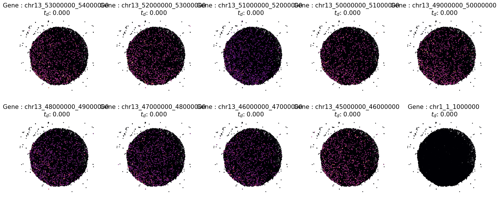
# Inspect detecition visually by using the "plot_profiles function for last 10 SVG
# Define a custom pltargs dictionary with plot style options
pltargs = dict(s = 5,
                cmap = "magma",
                edgecolor = 'none',
                marker = 'H',
                )

# plot the profiles
fig,ax = ut.plot_profiles(cnt = data.cnt.loc[:,tail_profiles],
                          crd = data.real_crd,
                          rank_values = times.loc[tail_profiles,:].values.flatten(),
                          pltargs = pltargs,
                          )