SpatialClustering_SpatialMetabolomicsData

This tutorial demonstrates how to identify spatial domains on spatial metabolomics data using Pysodb and Spaceflow.

The reference paper can be found at https://www.nature.com/articles/s41467-022-31739-w and https://cordis.europa.eu/project/id/634402.

Import packages and set configurations

# Use the Python warnings module to filter and ignore any warnings that may occur in the program after this point.
import warnings
warnings.filterwarnings("ignore")

# Scanpy (imported as sc) is a package for single-cell RNA sequencing analysis.
import scanpy as sc

# from SpaceFlow package import SpaceFlow module
from SpaceFlow import SpaceFlow

# Imports a palettable package
import palettable
# Create three variables with lists of colors for categorical visualizations and biotechnology-related visualizations, respectively.
cmp_pspace = palettable.cartocolors.diverging.TealRose_7.mpl_colormap
cmp_domain = palettable.cartocolors.qualitative.Pastel_10.mpl_colors
cmp_ct = palettable.cartocolors.qualitative.Safe_10.mpl_colors

When encountering the error “No module name ‘palettable’”, users need to activate conda’s virtual environment first at the terminal and run the following command in the terminal: “pip install palettable”. This approach can be applied to other packages as well, by replacing ‘palettable’ with the name of the desired package.

Streamline development of loading spatial data with Pysodb

# Import pysodb package
# Pysodb is a Python package that provides a set of tools for working with SODB databases.
# SODB is a format used to store data in memory-mapped files for efficient access and querying.
# This package allows users to interact with SODB files using Python.
import pysodb

# Initialize the sodb object
sodb = pysodb.SODB()

# Define names of the dataset_name and experiment_name
dataset_name = 'MALDI_seed'
experiment_name = 'S655_WS22_320x200_15um_E110'
# Load a specific experiment
# It takes two arguments: the name of the dataset and the name of the experiment to load.
# Two arguments are available at https://gene.ai.tencent.com/SpatialOmics/.
adata = sodb.load_experiment(dataset_name,experiment_name)

load experiment[S655_WS22_320x200_15um_E110] in dataset[MALDI_seed]

Perform SpaceFlow to spatial clustering for spatial metabolomics data

# Create SpaceFlow Object
sf = SpaceFlow.SpaceFlow(
    count_matrix=adata.X,
    spatial_locs=adata.obsm['spatial'],
    sample_names=adata.obs_names,
    gene_names=adata.var_names
)

When encountering the error “Error: The truth value of an array with more than one element is ambiguous. Use a.any() or a.all().” In the “SpaceFlow.py” file from the SpaceFlow package, the user is advised to make the following modifications within the init function. Replace “elif count_matrix and spatial_locs:” with “elif count_matrix is not None and spatial_locs is not None:”. Additionally, modify “if gene_names:” and “if sample_names:” to “if gene_names is not None:” and “if sample_names is not None:” respectively. The above modifications ensure that the if statement returns a single boolean value respectively.

# Preprocess data
sf.preprocessing_data()

When dealing with anndata (adata) where the count or expression matrix is extremely sparse, or where there are a very limited number of features (as is often the case with spatial proteomics data), it may be preferable to forego data preprocessing. This is because over-processing in these instances could lead to errors or diminished performance in downstream tasks. To skip preprocessing, user will need to make modifications to the preprocessing_data function within the “SpaceFlow.py” file of the SpaceFlow package. Specifically, user should comment out the sc.pp.normalize_total(), sc.pp.log1p(), and sc.pp.highly_variable_genes() functions.

When encountering the error “Error: You can drop duplicate edges by setting the ‘duplicates’ kwarg”, in “SpaceFlow.py” from the SpaceFlow package, modify the preprocessing_data function by: (1) removing target_sum=1e4 from sc.pp.normalize_total(); (2) changing the flavor argument to ‘seurat’ in sc.pp.highly_variable_genes(); (3) Save and rerun the analysis.

When encountering the error “Error: module ‘networkx’ has no attribute ‘to_scipy_sparse_matrix’”, users should first activate the virtual environment at the terminal and then downgrade NetworkX with the following command：”pip install networkx==2.8”. This will ensure that the correct version of NetworkX is installed within the specified virtual environment.

# Train a deep graph network model
embedding = sf.train(
    spatial_regularization_strength=0.1,
    z_dim=50,
    lr=1e-3,
    epochs=1000,
    max_patience=50,
    min_stop=100,
    random_seed=42,
    gpu=0,
    regularization_acceleration=True,
    edge_subset_sz=1000000
)

Epoch 2/1000, Loss: 34.639442443847656
Epoch 12/1000, Loss: 34.61619186401367
Epoch 22/1000, Loss: 34.61435317993164
Epoch 32/1000, Loss: 34.614418029785156
Epoch 42/1000, Loss: 34.61484909057617
Epoch 52/1000, Loss: 34.6142692565918
Epoch 62/1000, Loss: 34.611209869384766
Epoch 72/1000, Loss: 34.61259841918945
Epoch 82/1000, Loss: 34.61189651489258
Epoch 92/1000, Loss: 34.61252212524414
Epoch 102/1000, Loss: 34.61070251464844
Epoch 112/1000, Loss: 34.60990524291992
Epoch 122/1000, Loss: 34.61140823364258
Epoch 132/1000, Loss: 34.6107063293457
Epoch 142/1000, Loss: 34.61091232299805
Epoch 152/1000, Loss: 34.609031677246094
Epoch 162/1000, Loss: 34.60935974121094
Epoch 172/1000, Loss: 34.60832595825195
Epoch 182/1000, Loss: 34.60786437988281
Epoch 192/1000, Loss: 34.60796356201172
Epoch 202/1000, Loss: 34.60761642456055
Epoch 212/1000, Loss: 34.60805130004883
Epoch 222/1000, Loss: 34.60633850097656
Epoch 232/1000, Loss: 34.60551071166992
Epoch 242/1000, Loss: 34.60599899291992
Epoch 252/1000, Loss: 34.606834411621094
Epoch 262/1000, Loss: 34.604793548583984
Epoch 272/1000, Loss: 34.604347229003906
Epoch 282/1000, Loss: 34.603111267089844
Epoch 292/1000, Loss: 34.60285568237305
Epoch 302/1000, Loss: 34.602264404296875
Epoch 312/1000, Loss: 34.601409912109375
Epoch 322/1000, Loss: 34.600948333740234
Epoch 332/1000, Loss: 34.60084915161133
Epoch 342/1000, Loss: 34.602237701416016
Epoch 352/1000, Loss: 34.59991455078125
Epoch 362/1000, Loss: 34.60015106201172
Epoch 372/1000, Loss: 34.59867858886719
Epoch 382/1000, Loss: 34.59828567504883
Epoch 392/1000, Loss: 34.59810256958008
Epoch 402/1000, Loss: 34.59739303588867
Epoch 412/1000, Loss: 34.59801483154297
Epoch 422/1000, Loss: 34.59721374511719
Epoch 432/1000, Loss: 34.597496032714844
Epoch 442/1000, Loss: 34.59624099731445
Epoch 452/1000, Loss: 34.595703125
Epoch 462/1000, Loss: 34.59564971923828
Epoch 472/1000, Loss: 34.595947265625
Epoch 482/1000, Loss: 34.59563446044922
Epoch 492/1000, Loss: 34.59565734863281
Epoch 502/1000, Loss: 34.59561538696289
Epoch 512/1000, Loss: 34.594581604003906
Epoch 522/1000, Loss: 34.59492492675781
Epoch 532/1000, Loss: 34.59452438354492
Epoch 542/1000, Loss: 34.59488296508789
Epoch 552/1000, Loss: 34.59366226196289
Epoch 562/1000, Loss: 34.59366989135742
Epoch 572/1000, Loss: 34.593658447265625
Epoch 582/1000, Loss: 34.593902587890625
Epoch 592/1000, Loss: 34.59398651123047
Epoch 602/1000, Loss: 34.59341812133789
Epoch 612/1000, Loss: 34.594024658203125
Epoch 622/1000, Loss: 34.5934944152832
Epoch 632/1000, Loss: 34.5926399230957
Epoch 642/1000, Loss: 34.5951042175293
Epoch 652/1000, Loss: 34.593170166015625
Epoch 662/1000, Loss: 34.59335708618164
Epoch 672/1000, Loss: 34.59296798706055
Epoch 682/1000, Loss: 34.59357452392578
Epoch 692/1000, Loss: 34.593448638916016
Epoch 702/1000, Loss: 34.5923957824707
Epoch 712/1000, Loss: 34.592681884765625
Epoch 722/1000, Loss: 34.59284210205078
Epoch 732/1000, Loss: 34.592811584472656
Epoch 742/1000, Loss: 34.59242630004883
Epoch 752/1000, Loss: 34.59189224243164
Epoch 762/1000, Loss: 34.59220504760742
Epoch 772/1000, Loss: 34.59148025512695
Epoch 782/1000, Loss: 34.59242248535156
Epoch 792/1000, Loss: 34.591590881347656
Epoch 802/1000, Loss: 34.59206008911133
Epoch 812/1000, Loss: 34.5922737121582
Epoch 822/1000, Loss: 34.59100341796875
Epoch 832/1000, Loss: 34.590911865234375
Epoch 842/1000, Loss: 34.59068298339844
Training complete!
Embedding is saved at ./embedding.tsv

# Save the embeddings of the trained SpaceFlow model to adata.obsm['SpaceFlow'].
adata.obsm['SpaceFlow'] = embedding

# Calculate the nearest neighbors in the 'SpaceFlow' representation and computes the UMAP embedding.
sc.pp.neighbors(adata, use_rep='SpaceFlow')
sc.tl.umap(adata)

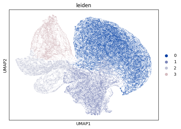
# Perform a Leiden clustering.
sc.tl.leiden(adata, resolution=0.04, key_added='leiden')

# Plot a UMAP embedding.
sc.pl.umap(adata, color= 'leiden', color_map= cmp_pspace)

# Display a spatial embedding plot with clustering information.
ax = sc.pl.embedding(adata, basis= 'spatial', color='leiden', show= False, color_map=cmp_pspace)
ax.axis('equal')

(-14.950000000000001, 335.95, -8.950000000000001, 209.95)