Application with new data (3D)

This tutorial demonstrates spatial clustering on 3D mouse visual cortex data using Pysodb.

A reference paper can be found at https://www-science-org.ezproxy.is.ed.ac.uk/doi/full/10.1126/science.aat5691.

Import packages and set configurations

[1]:

# Use the Python warnings module to filter and ignore any warnings that may occur in the program after this point.
import warnings
warnings.filterwarnings("ignore")

[2]:

# scanpy (imported as sc) is a package for single-cell RNA sequencing analysis
import scanpy as sc
# matplotlib.pyplot (imported as plt) is a package for data visualization
import matplotlib.pyplot as plt

[3]:

# Import STAGATE_pyG package
import STAGATE_pyG as STAGATE

If users encounter the error “No module named ‘STAGATE_pyG’” when trying to import STAGATE_pyG package, first ensure that the “STAGATE_pyG” folder is located in the current script’s directory.

[4]:

# Imports a palettable package
import palettable
# Define three color maps, a diverging color map (cmp_pspace), and two qualitative color maps (cmp_domain and cmp_ct)
cmp_pspace = palettable.cartocolors.diverging.TealRose_7.mpl_colormap
cmp_domain = palettable.cartocolors.qualitative.Pastel_10.mpl_colors
cmp_ct = palettable.cartocolors.qualitative.Safe_10.mpl_colors

When encountering the error “No module name ‘palettable’”, users need to activate conda’s virtual environment first at the terminal and run the following command in the terminal: “pip install palettable”. This approach can be applied to other packages as well, by replacing ‘palettable’ with the name of the desired package.

Streamline development of loading spatial data with Pysodb

[5]:

# Import pysodb package
# Pysodb is a Python package that provides a set of tools for working with SODB databases.
# SODB is a format used to store data in memory-mapped files for efficient access and querying.
# This package allows users to interact with SODB files using Python.
import pysodb

[6]:

# Initialization
sodb = pysodb.SODB()

[7]:

# Define names of the dataset_name and experiment_name
dataset_name = 'Wang2018three'
experiment_name = 'data_3D'
# Load a specific experiment
# It takes two arguments: the name of the dataset and the name of the experiment to load.
# Two arguments are available at https://gene.ai.tencent.com/SpatialOmics/.
adata = sodb.load_experiment(dataset_name,experiment_name)

load experiment[data_3D] in dataset[Wang2018three]

Data processing

[8]:

#Normalization
sc.pp.highly_variable_genes(adata, flavor="seurat_v3", n_top_genes=3000)
sc.pp.normalize_total(adata, target_sum=1e4)
sc.pp.log1p(adata)

When encountering the Error “Please install skmisc package via ‘pip install –user scikit-misc’”, users can follow the provided instructions: activate the virtual environment at the terminal, execute “pip install –user scikit-misc”, and then restart the kernel to ensure the package is properly installed and available for use.

[9]:

adata.obsm['spatial_3D'] = adata.obs[['x','y','z']].values

Constructing the spatial network with diverse rad_cutoff

[10]:

# Define a list with different radius cutoff values
rad_cutoff_list = [15,20]
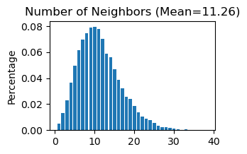
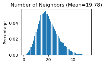
# Consturcting network for different radius cutoff
for rad_cutoff in rad_cutoff_list:
    STAGATE.Cal_Spatial_Net(adata, rad_cutoff=rad_cutoff)
    STAGATE.Stats_Spatial_Net(adata)
    adata = STAGATE.train_STAGATE(adata)
    adata.obsm[f'STAGATE_rad{rad_cutoff}'] = adata.obsm['STAGATE'].copy()
# Save the adata object
adata.write_h5ad('3D_spatialnet_h5ad')

------Calculating spatial graph...
The graph contains 369952 edges, 32845 cells.
11.2636 neighbors per cell on average.
Size of Input:  (32845, 28)

100%|██████████| 1000/1000 [00:27<00:00, 35.91it/s]

------Calculating spatial graph...
The graph contains 649580 edges, 32845 cells.
19.7771 neighbors per cell on average.
Size of Input:  (32845, 28)

100%|██████████| 1000/1000 [00:43<00:00, 22.99it/s]

../_images/Spatial_clustering_Application_with_new_data_%283D%29_18_4.png

../_images/Spatial_clustering_Application_with_new_data_%283D%29_18_5.png

Clustering and UMAP

rad_cutoff=15

[11]:

# Calculate the nearest neighbors in the 'STAGATE_rad15' representation and computes the UMAP embedding.
sc.pp.neighbors(adata, use_rep='STAGATE_rad15')
sc.tl.umap(adata)
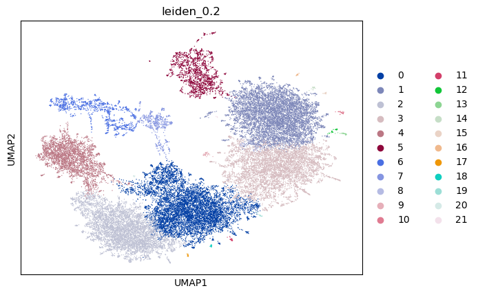
# Perform a Leiden clustering with 'STAGATE_rad15' representation, and add a key_added as 'leiden_0.2'
sc.tl.leiden(adata,resolution=0.2,key_added='leiden_0.2')

When encountering the Error “Please install the leiden algorithm: ‘conda install -c conda-forge leidenalg’ or ‘pip3 install leidenalg’”, users can follow the provided instructions: activate the virtual environment at the terminal, execute “pip3 install leidenalg”.

[12]:

# Plot a UMAP embedding ('STAGATE_rad15') colored 'leiden_0.2'
sc.pl.umap(adata, color='leiden_0.2')

../_images/Spatial_clustering_Application_with_new_data_%283D%29_23_0.png

[13]:

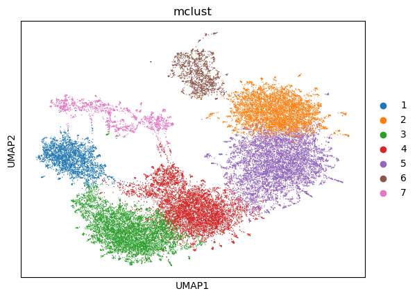
# Perform mclust clustering with 'STAGATE_rad15' representation, and set 'num_cluster' to 7
adata = STAGATE.mclust_R(adata, used_obsm='STAGATE_rad15', num_cluster=7)

R[write to console]:                    __           __
   ____ ___  _____/ /_  _______/ /_
  / __ `__ \/ ___/ / / / / ___/ __/
 / / / / / / /__/ / /_/ (__  ) /_
/_/ /_/ /_/\___/_/\__,_/____/\__/   version 6.0.0
Type 'citation("mclust")' for citing this R package in publications.

fitting ...
  |======================================================================| 100%

[14]:

# Plot a UMAP embedding ('STAGATE_rad15') colored 'mclust'
sc.pl.umap(adata, color='mclust')

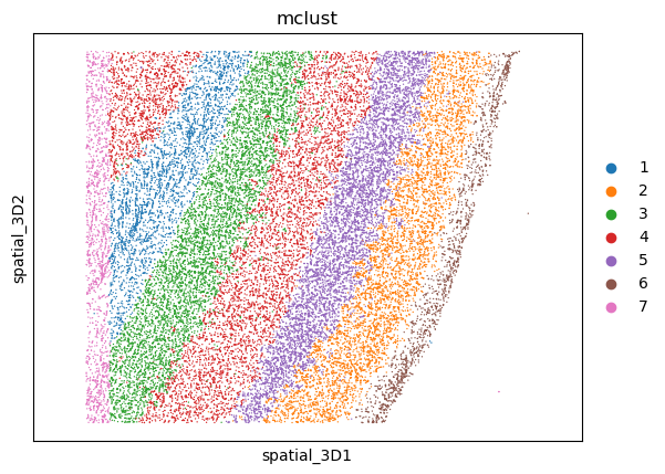
../_images/Spatial_clustering_Application_with_new_data_%283D%29_25_0.png

[15]:

# Plot a spatial distribution ('STAGATE_rad15') base on 'spatial_3D' with 'mclust' clustering
ax = sc.pl.embedding(adata, basis='spatial_3D',color='mclust',show=False)
# Ensure a consistent aspect ratio along all three dimensions
ax.axis('equal')

[15]:

(-78.95, 1899.95, -64.7, 1600.7)

../_images/Spatial_clustering_Application_with_new_data_%283D%29_26_1.png

rad_cutoff=20

[16]:

# Calculate the nearest neighbors in the 'STAGATE_rad15' representation and computes the UMAP embedding.
sc.pp.neighbors(adata, use_rep='STAGATE_rad20')
sc.tl.umap(adata)
# Perform a Leiden clustering with 'STAGATE_rad20' representation, and add a key_added as 'leiden_0.2'
sc.tl.leiden(adata,resolution=0.2,key_added='leiden_0.2')

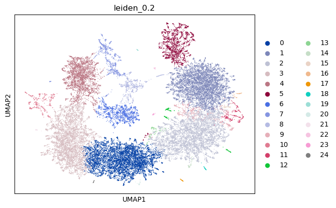
[17]:

# Plot a UMAP embedding ('STAGATE_rad20') colored 'leiden_0.2'
sc.pl.umap(adata, color='leiden_0.2')

../_images/Spatial_clustering_Application_with_new_data_%283D%29_29_0.png

[18]:

# Perform mclust clustering with 'STAGATE_rad20' representation, and set 'num_cluster' to 9
adata = STAGATE.mclust_R(adata, used_obsm='STAGATE_rad20', num_cluster=9)

fitting ...
  |======================================================================| 100%

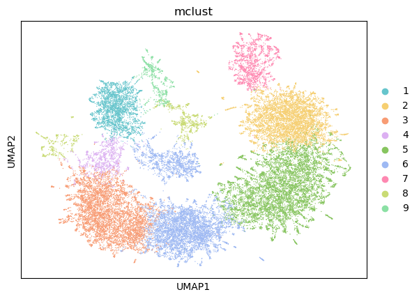
[19]:

# Plot a UMAP embedding ('STAGATE_rad20') colored 'mclust'
sc.pl.umap(adata, color='mclust',palette=cmp_domain)
#plt.savefig('../figures/spatialclustering/3D_umap.png',dpi=400,transparent=True,bbox_inches='tight')

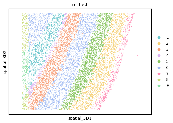
../_images/Spatial_clustering_Application_with_new_data_%283D%29_31_0.png

[20]:

# Plot a spatial distribution ('STAGATE_rad20') base on 'spatial_3D' with 'mclust' clustering
ax = sc.pl.embedding(adata, basis='spatial_3D',color='mclust',palette=cmp_domain,show=False)
# Ensure a consistent aspect ratio along all three dimensions
ax.axis('equal')
#plt.savefig('../figures/spatialclustering/3D_spatial.png',dpi=400,transparent=True,bbox_inches='tight')

[20]:

(-78.95, 1899.95, -64.7, 1600.7)

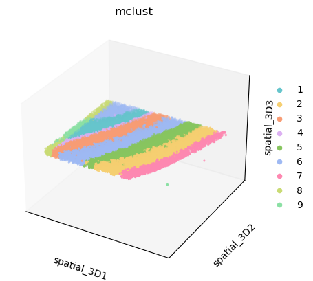
../_images/Spatial_clustering_Application_with_new_data_%283D%29_32_1.png

[21]:

# Plot a spatial distribution ('STAGATE_rad20') base on 'spatial_3D' with 'mclust' clustering to project in a 3D space
ax = sc.pl.embedding(adata, basis='spatial_3D',color='mclust', projection='3d',palette=cmp_domain,show=False)
# Ensure a consistent aspect ratio along all three dimensions
ax.axis('equal')

[21]:

(-78.95000000000016,
 1899.9500000000003,
 -221.45000000000016,
 1757.4500000000003)

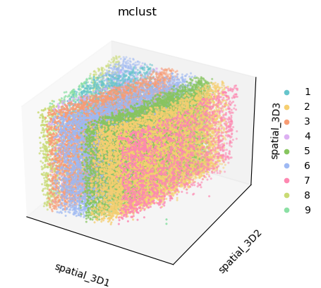
../_images/Spatial_clustering_Application_with_new_data_%283D%29_33_1.png

[22]:

# Plot a spatial distribution ('STAGATE_rad20') base on 'spatial_3D' with 'mclust' clustering for for enhanced visualization
sc.pl.embedding(adata, basis='spatial_3D',color='mclust', projection='3d',palette=cmp_domain,show=False)

[22]:

<Axes3D: title={'center': 'mclust'}, xlabel='spatial_3D1', ylabel='spatial_3D2', zlabel='spatial_3D3'>

../_images/Spatial_clustering_Application_with_new_data_%283D%29_34_1.png

[23]:

# Save the result object
adata.write_h5ad('3D_mclust.h5ad')